Executive Summary
Setting a proper time horizon is a crucial step in planning for retirement, and is typically done by making a reasonably conservative estimate of life expectancy... perhaps with a few extra years for padding, depending on a client's preferences.
Yet in many cases, planners adopt a uniform "standard" assumption for clients, without adapting it to even the most basic client circumstances, like whether the client is a single person or a married couple, despite the material difference between individual and joint life expectancies. Similarly, while the reality is that there's a high likelihood that a married couple will live several decades in retirement, the odds are overwhelming that for much of that time period, only one - but not both - of them will be alive.
As a result, it may be time for planners to begin to adopt more nuanced life expectancy assumptions for clients, at a minimum making a distinction between individuals and married couples, and with reductions in the later years for married couples to acknowledge the fact that while it's likely one may be alive, it's very unlikely that both will live through the entire time horizon. Otherwise, simply choosing an arbitrarily long time horizon for clients, paired with a high standard of Monte Carlo success, may actually result in an unnecessarily constrained retirement lifestyle!
Life Expectancy Planning For Singles Vs Couples
While the "default" retirement assumption is often based on a married couple, the reality is that often planning involves a single individual, whether unmarried or a widow. Yet the reality is that the "typical" retirement assumption of a 30-year time horizon at age 65 looks drastically different in the context of a married couple versus a single person, as shown in the chart below:
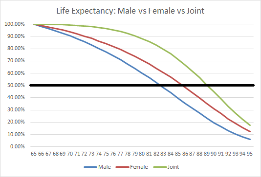
The black horizontal line represents the 50th percentile for survival (or what we commonly call "life expectancy"), which is approximately age 89 for the starting-age-65 couple (based on the Social Security Administration's 2007 Period Life Table). Notably, though, it's only age 85 for a 65-year-old female, and age 82 for a 65-year-old single male. This is not a trivial difference; the life expectancy for a single person is 4-7 years shorter than for a married couple, and it's only 24 years in the first place for a 65-year-old married couple. In other words, the life expectancy when planning for individuals is 15%-30% shorter, which - if properly adjusted - would allow for a significant increase in retirement spending!
Of course, many planners don't like to use life expectancy alone as a basis for planning - after all, by definition half the clients will live longer - which is why age 95 is not uncommon as a final retirement age for a married couple. Yet here, again, the difference between couples and singles is notable; there is only a 12% chance for the single female to still be alive, and a 6% chance for the single male, but a (comparatively) whopping 18% chance that at least one member of the couple is alive at age 95.
A Deeper Look At Joint Life Expectancies
As just noted, the joint life expectancy for a 65-year-old couple is age 89, though by age 95 the survival probability rapidly falls from 50% to only 18%. However, it's important to bear in mind that the life expectancy survival probabilities for a married couple are based on the likely that they're not both deceased - or viewed another way, the couple can meet the condition of "still alive" as long as one, the other, or both are alive.
When viewed in component parts, though, this distinction between the probability that only one member of the couple is alive, versus both are alive, is significant, as shown in the chart below:
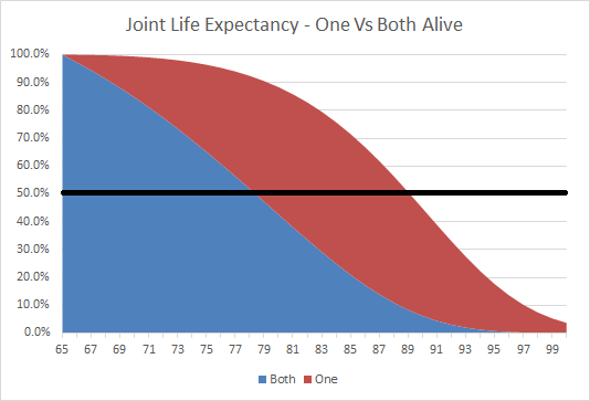
Once again, the black horizontal line represents the 50th percentile. While the "stacked" probability of having both or one alive once again confirms the age 89 life expectancy of the couple, the startling reality is that the 50th percentile of having both alive is only age 78! In fact, at age 89, while there may be a 50% probability that at least one member of the couple is alive, the odds are only about 8% that it's both of them and a whopping 42% that it's one - and only one - of them still alive.
For those who "conservatively" plan for a longer time horizon, again there is an 18% probability that at least one member of the couple is still alive at age 95. However, that's based on a probability of about 17% that only one of them is alive, and a less-than-1% chance that both of them are still alive!
Practical Financial Planning Implications
The practical implications of these life expectancy probability charts are relatively straightforward - that routinely planning for all 65-year-old clients to live for 30 years to age 95 may actually be remarkably conservative, and possibly too conservative.
Granted, it's worth noting that the Social Security Administration's Period Life tables are only one of several commonly used life expectancy tables, which also include the U.S. Life Tables from the U.S. Census and the Annuity 2000 tables from the Society of Actuaries, both of which tend to assume slightly greater longevity. And for those who are optimistic on the impact of advances in medical technologies, none of the tables may necessarily fully account for how life expectancy could change in the future (on the other hand, it's not clear whether today's retirees may live long enough to witness a material change in the life expectancy for seniors).
Nonetheless, the point remains that, to the extent planners do choose "some" baseline as a planning time horizon for married couples, arguably a distinctly different - and shorter - time horizon should be used when planning for a single individual. To use the same arbitrary planning time horizon for individuals and married couples belies the material differences in longevity that exist.
In addition, the reality remains that there is an even more significant difference between the probability that one member of a couple remains alive, versus the probability that both remain alive, despite the fact that a "joint life expectancy" inherently includes both. When evaluated based on the component parts, it becomes clear that even for planners who wish to make a conservative longevity assumption, proper planning should include a material time period where only one member of the couple is alive, with spending adjusted accordingly.
Of course, given that some household expenses are fixed, the death of one member of the couple doesn't necessarily mean that spending falls by 50%; nonetheless, baseline spending when just one member of a married couple is alive is clearly some amount materially lower than when both are alive (not to mention how spending may simply decline in later years as lifestyle slows down as well). Either way, between lifestyle declines and the death of one spouse, it seems difficult to justify not making a material reduction real spending in the final years of a retirement projection for a married couple.
An alternative solution to deal with this challenge is to do Monte Carlo retirement projections assuming "stochastic" life expectancy - in other words, in every trial of the retirement plan with various dynamic probability-based random returns, also use dynamic probability-based life expectancy. From a practical perspective, not all financial planning and Monte Carlo software can do this, though. In addition, the reality is that if life expectancy is modeled with randomness, recommended spending levels may actually be slightly higher than just arbitrarily assuming a long time horizon past life expectancy; after all, with stochastic life expectancy, sometimes a client's "irresponsibly high" spending behaviors will be justified by a "bad luck" early death. On the other hand, this is also an implicit acknowledgement that assuming an arbitrarily fixed long time horizon, plus requiring a high probability of success, can actually result in an ultra-extreme-conservative retirement projection that may unnecessarily constrain retirement spending to protect against miniscule risks.
The bottom line, though, is simply this: when setting a time horizon for a retirement plan, there should be differences in the planning assumptions for single individuals versus married couples. In addition, it's crucial to recognize that while there is a high likelihood that at least one member of a couple lives for several decades in retirement, the odds are also very high that it will be only one of them for much of that time period - not both - so be certain to plan and adjust projected retirement expenses accordingly! And of course, if individual client circumstances dictate, you may want to make further client-specific life expectancy adjustments as well!
Larry Frank says
A great post Michael that gets to mental heuristic shortcuts
(http://en.wikipedia.org/wiki/Heuristic) the profession has migrated to as
opposed to number crunching with client specifics in mind.
You briefly mention Monte Carlo (MC) simulations that dynamically
adjust stochastic remaining life expectancy within the simulation each year – a
topic near and dear to my heart via work with co-researchers Mitchell and
Blanchett. The idea is that modeling should more closely reflect real life and
how remaining life expectancy slowly changes (currently about 3 to 4 month
increase in distribution period with each year aged) is slowly being adopted …
well ahead of software to no surprise since software is a result of demand
based on thoughts and concepts.
When this combination of Probability of the Portfolio (risk
and return characteristics) is combined with Probability of the Person
(longevity table characteristics) within annually updating stochastic modeling,
one quickly sees how previous spending affects later portfolio values – and
what factors do impact retaining that portfolio (dynamic allocation adjustments
too) for income generation into superannuated ages.
You see, annually updating facts more closely resembles
annual reviews than running a single MC simulation over some ill-defined time
period. Software demand to do that hasn’t caught up because we as practitioners
aren’t demanding software to more closely reflect how annual reviews actually
work. Of course, we don’t know future returns – precisely what MC simulations
exist to provide a sense of the range of possibilities. However, actual annual
reviews do incorporate actual changes to data, both historical and expected, as
well as updating period life tables. Thus, the annual review is more important
than the annual simulation since it incorporates now known facts and data
unknown just a year earlier.
I think it is great that you periodically remind readers that the first and key consideration is the time period in question … this has a tremendous influence on results, even more so than risk and return characteristics if I’d be so bold to state.
An interesting article; enough so that I ran a few quick scenarios to see what difference it made for my spouse and me (no children or bequest goals). While it would reduce expenses earlier than in our current model, the adjustment permits only a very small (2-3%) annual spending increase at the beginning of retirement.
So, it does make a difference but, seemingly, not a big enough one to fret over during a 30+ yr retirement.
It is very hard to discern how this works by comparing how much one could take out of their portfolio under any method. This leads to an erroneous conclusion that the method that allows more is better than the method that suggests one should take out less – right now. This is because single-point comparisons don’t do a good job evaluating total lifetime cash flow. When you sum up potential cash flows you begin to see how early high spending results in future lower spending using the same risk and reward characteristics for comparison. Caution on then concluding that riskier portfolios lead to greater cash flow … it doesn’t work that way: what returns give, volatility in returns takes away.
Agree regarding being cautious about conclusions from “a few quick scenarios.” But, it wasn’t a single point comparison. I did some FIRECalc runs to quantify (monetize) the practical implication to spending of adjustments to life expectancy. The result was that while the late life impact may be large in any one year, the impact on early retirement spending is negligible. That result makes intuitive sense to me as well. In fact, one almost doesn’t need to do the math. So, again, it doesn’t seem to make much difference from a practical standpoint.
For this time period based on today’s ages. However, dynamic updating of the distribution period based on ages recognizes that the distribution period doesn’t go down one year at a time until you hit age 88 for example. That end age also slowly extends to an older age … one never reaches their expected longevity age based on current age because it is always older than your presently are. Dynamic updating also means that the slow process of people living longer gets incorporated into the life tables over time. Thus, the expected longevity of someone in their 70’s today is younger than expected longevity of someone in their 70’s a decade from now. I’m not sure if FIRECalc actually adjusts longevity for each age “to longevity” since that age slowly gets older as one gets older.
It is very difficult to discern differences between distribution outcomes just by their first year comparisons. Rather, the sums of the lifetime cash flows should be compared. This simulates annual reviews when a series of simulations are strung together replicating aging by one year and also adjusting the expected lifetime age using the older age each year. This process brings out the effect of spending, as well as risk and return characteristics, better.
Indeed a good start. @MichaelKitces We superimposed portfolio on the life expectancy graph with case studies (plural) http://bit.ly/1hqB2TW We use white collar actuarial tables in calculating the probabilities on our longevity graphs. The case studies help a lot.
Michael,
Do you have any suggested software to handle the life expectancy based MC modelling? I am not sure if MGP can be adapted to do this, but I will look into it. Also, should we add a few questions on our client data gathering forms about family longevity? I have had a few clients who specifically stated concerns about their expected long or short longevity, and wanted that figured into their plans.
Michael,
Great educational post. But while you are on the topic of moving advisors in the right direction on longevity planning, I say it’s also time that we simply stop using the Social Security Administration Period Life Tables for studying longevity. That data is the easiest to get, but it also dramatically underestimates lifespans for financial planning clients for two reasons:
-it’s for the aggregate population, but the people reading your posts will have above average longevity
-it’s a period life table rather than a cohort life table. To calculate the probability a 65 year old lives to 95, it uses the 2007 mortality rates for ages 65-95. But by the time today’s 65 year old gets to 75 or 85, their mortality rates will be lower. Mortality continues to gradually improve in a rather consistent way, and just this issue alone could lead to life expectancy underestimates for 65 year olds to be in the neighborhood of 3 years.
I agree in principle Wade about the use of tables. However, by the time the 65 year old gets to 75 or 85, any table will also have been updated – the use of the 2007 table will have shifted to the 2017 or 2027 table respectively as the retiree ages; thus, capturing the effect of improved life expectancy for this important question about what it should be for THOSE remaining expected years when those years are eventually reached.
The overall effect of longevity extension overtime is to slowly adjust the distribution period to longer periods and thus slowly adjusting the withdrawal rate down relative to what it might have been using a static table to establish the distribution periods. To the retiree it would be imperceptible – example, would I remember what my distribution rate would have been now compared to what it was projected to be 10 years ago using the 1997 tables?
The all important annual review is to capture updated data which is ALL stochastic in nature. Results of simulations are indicative, not predictive, of feasibility at only the moment in time the simulation is run. Before retiring as an Air Force pilot flying internationally, we’d have the flight plan. But, we needed to continually update progress to make course adjustments for winds different than planned and thus the effect on fuel usage and how weather may have changed while enroute to the destination. It didn’t matter what we planned to use fuel wise, but what we actually had remaining compared to what we needed at any point along the way.
Michael, would it be valid/valuable to multiply 100% minus the Monte Carlo probability by the “one or the other alive still alive” probability to come up with a probability of failure. Money Tree Golden Years provides four different probabilities, one for the full LE age and one for that age minus 5, 10 and 15 years. If we subtract these from 100% (to get the monte carlo probability of failure) and multiply this number by the “one or the other alive” probability does this usefully factor in the LE probabilities?
Thanks,
Kay
I disagree that planning for both spouses to live to age 95 is the most conservative case. In many cases, the most conservative case financially is to assume an early death for one spouse followed by a long widowhood for the other spouse.
Here are some of the considerations that have to taken into account:
1) Expenses do not decrease in half when one spouse dies. Housing and transportation, for example, are not reduced in half.
2) SS income may be cut in half if both spouses had similar earnings histories.
3) Pension income may be lost if there is no survivor benefits for the current spouse. This is increasingly common with the increase in divorce and second marriages.
4) Tax rates go from married filing joint to single filing status. This has a huge impact on taxes paid, especially after RMDs kick in.
I urge planners to run analyses assuming both have long lives as well as the case in which one predeceases the other by a significant time period. In our personal case, we found that the early widowhood case had a much greater financial risk than the case of both living to 95.
wrong both have over 100 thousand in bank and one was in milatary so one gets a check from milatary and the other one gets his check if he dies first but both
I never believe in miracle until I experienced one sometime ago and it really worked for me.I was in love with this guy and he is in love with me too for 3years and we making preparations to get married but to my surprise, he got engaged with another girl. I was about loosing my man to another lady under the influence, until I met _____________(Robinsonbuckler@ hotmail. com) on net that claimed he can help me out.He helped me bring my lover back and after some few days i noticed that my man came back to me with so much love for me. We are happily back now. people with similar problems can contact him……
Such an important topic, Michael, and such great insight. Thank you!
I’ve been playing around with the OpenSocialsecurity.com calculator, which includes the ability to either choose a mortality table from a few different 2017 ones; or simply put in your own mortality age assumptions.
While not quite stochastic MC mortality planning, it does at least one to run run a variety of scenarios to see how claiming SSA at different ages affects total lifetime NPV of SSA payments.
Would love to see an update of this article or maybe a follow on that looks at using the Open Social Security calculator to do some modeling, and provide some advice on which mortality scenarios to test.