Executive Summary
With the rise of Monte Carlo analysis as the most commonly used method of conducting retirement projections for clients, 'probability of success' has become the focal point for communicating retirement preparedness to clients. While a number of issues with framing results around probability of success have been noted – from not accounting for the magnitude of failure, to not acknowledging that small 'adjustments' can often save a 'failing' plan, and even some biases related to how we think about 'wrong' probabilistic forecasts – there is an additional issue with the current usage of Monte Carlo analyses that has gone largely unnoticed: If you are doing ongoing planning for a client who is willing to adjust their spending, then the norms that have emerged – particularly strong negative perceptions of planning results below 70% probability of success – may not be as problematic as most advisors (and clients!) think. In fact, a 50% probability of success (or lower!) may be reasonable for retirees who are willing to make spending adjustments.
One concern when reporting Monte Carlo results to a client framed around ‘probability of success’ is that anything less than 100% can sound scary. Consider a 50% probability of success: ‘Failing’ one-out-of-two times when failure implies running out of money in retirement simply does not sound acceptable. Such a result can make clients feel that they are unprepared for retirement and that they must save even more or retire even later so that they can achieve a higher probability of success. It is important, however, to think carefully about what a 50% result actually implies. First, this metric alone actually tells us nothing about how severe 'failure' is. If 90% of a client's desired income comes from guaranteed income sources, then 'failure' is capped at a relatively modest 10% cut in a client's income, which is not ideal but far from devastating. Moreover, adjustments can often save a 'failing' plan, so simply shifting a 50% probability of success framing to a 50% probability of adjustment can take a lot of sting out of that result.
Additionally, the difference between setting spending based on a one-time projection versus ongoing projections should be acknowledged, as these two approaches are fundamentally very different. If you only had one opportunity to select a spending level and you were forced to stick with that no matter what happened in the future, then selecting a spending level with a 95% (or higher) probability of success may make a lot of sense. But the reality is that planners generally provide ongoing projections for clients, and even those who provide one-time plans will recommend periodic updates. And if a retiree is going to keep their plan up to date (which allows for opportunities to identify when a plan is veering off course and adjust as needed), then planning to a 50% probability of success (i.e., a plan that needs to be adjusted one-out-of-two times) is not nearly as scary. Furthermore, it should be noted that a 50% probability of success means adjustment at any point in time in the future, and not necessarily even an adjustment in the near future.
To examine what planning using lower probability of success levels actually looks like, we compare planning outcomes using spending levels continually adjusted to maintain a constant 95%, 70%, 50%, and 20% probability of success throughout retirement using actual historical outcomes going back to 1871. What may be surprising is that we find that median, minimum, and maximum spending levels throughout 30-year retirement periods are actually quite consistent regardless of the probability of success used! In other words, if you are going to adjust spending on an ongoing basis, then returns experienced end out being the largest factor in determining how much can be spent, with income shaded either slightly higher (lower probability of success) or lower (higher probability of success) based on the success level targeted. Where we do see larger differences (although still smaller than many might anticipate) is with respect to terminal wealth levels, which suggests that when using Monte Carlo analyses for ongoing clients, the probability of success level targeted is actually more about a trade-off between income and legacy than any genuine difference in the risk that a portfolio will be depleted.
Since our intuitions generally tell us that a 50% probability of success is insufficient, advisors may wish to further consider how Monte Carlo results are framed to clients. Presenting clients with a range of potential strategy considerations may be beneficial in helping explore what best fits a client's preferences. Furthermore, advisors should give thought specifically to what probability of success level best balances the trade-off between income and legacy for a client. Unfortunately, current planning tools do not make illustrating these types of dynamic strategies easy, but ultimately, the key point is that choosing a probability of success level to use is not as simple as being able to apply a one-size-fits-all rule or a natural tilt toward being 'conservative' for the sake of not running out of money. For those retirees who are willing and able to make needed adjustments along the way, a 50% (or lower!) probability of success may provide a better result than most advisors (and clients) realize!
With the rise of Monte Carlo analysis as the most commonly used method of conducting financial planning analyses for clients, ‘probability of success’ has become the dominant metric that financial advisors rely on to assess and report a client’s prospects for financial security in retirement. It is the focal point of communicating results in most planning software. Often advisors build a plan, double-check their inputs, then load the results to see where the Monte Carlo gauge lands in terms of probability of success.
Imagine you are meeting with a client and putting together a plan for the first time. You are already feeling a little unsettled about their results, as your gut is telling you their spending is higher than you usually see with plans that have a strong probability of success. You check the results, and… 50%. How do you feel? How does this make your client feel?
If you are like most advisors, the result probably isn’t what you like to see. A recent study of mine (currently unpublished) found that approximately 90% of advisors felt it was not prudent to endorse a plan with a success probability of less than 70% for a fairly standard retiree client.
And for clients, the results can feel devastating. “So you’re saying that there’s a 50/50 chance that I will run out of money in retirement?”
Yet while a 50% probability of success sounds scary, in practice a 50% probability of success is probably much better than most advisors think! As while many limitations of presenting Monte Carlo results as “probability of success” have been noted (e.g., probability of adjustment better conveys the actual consequences, and dealing with the ‘wrong side of maybe’ fallacy), an even more fundamental issue exists: the norms that have developed around what is a ‘reasonable’ probability of success to target in the first place are flawed.
An Incomplete Monte Carlo Picture: Probabilities Of Success Without Magnitudes Of Failure?
A major issue with just reporting a Monte Carlo retirement plan’s ‘probability of success’ is that anything less than 100% sounds scary to clients (and advisors). ‘Failing’ one-out-of-two times – or even one-out-of-ten times – when failure implies destitution, poverty, and other running-out-of-money-in-retirement synonyms, simply does not sound acceptable. It is easy to understand how clients could see a result like this and feel that they are unprepared for retirement and that they must save even more or retire even later to get the success rate even more (safely) higher.
However, the reality is that often all it takes are minor adjustments to save a ‘failing’ plan, and the need to ‘adjust’ one-out-of-two times is fundamentally a very different takeaway. Simply put, if we say there’s a 50% probability of ‘failure’, it sounds potentially catastrophic; if we say there’s a 50% probability of adjustment, it doesn’t sound so bad. It just leads to the next natural question: What kind of ‘adjustment’ are we talking about?
In other words, clients who simply see a probability of success – and an implied risk of failure of falling off the rope – still may not know whether they are walking a tightrope six inches or sixty feet off of the ground. And that is a problem for coming to the right conclusions about how prepared one really is for retirement.
Example 1. Suppose George and Susan’s target spending is $6,000/month, and they are jointly receiving $5,500/month in Social Security. Which means they only actually rely on their portfolio for $500/month of spending!
Thus, their downward spending adjustment – if their portfolio were to run out altogether – is capped at ($6,000 – $5,500) ÷ $6,000 = 8.3% of their current lifestyle.
The ‘failure’ outcome, even if it does occur, is really just a modest adjustment in practice.
By contrast, if Jerry and Elaine’s target spending is also $6,000/month and they have no Social Security or other secure income streams (i.e., they are entirely reliant on their portfolio for income), then their spending adjustment (in theory) could go down ($6,000 – $0) ÷ $6,000 = 100%.
Based on how ‘failure’ is defined in a Monte Carlo analysis (i.e., depleting one’s assets without funding all of their goals), it is entirely possible that George and Susan’s plan could have a 50% probability of success or lower, yet not be a big deal given that they’ve effectively guaranteed that their reduction in spending would only be 8% for as long as they live. In other words, even if the couple spends their entire portfolio, it really would not be something they should spend much time stressing about, because the potential magnitude of adjustment is very small.
By contrast, Jerry and Elaine’s situation is much different. Depleting their portfolio without any guaranteed income sources would mean that their lifestyle could decline dramatically or outright catastrophically. The magnitude of Jerry and Elaine’s prospective failure, and the lifestyle adjustment it would entail, is far more extreme than that of the first couple, in a manner that isn’t conveyed by just looking at the probability of success alone. Jerry and Elaine would likely require a significantly higher probability of success to be comfortable because the magnitude of the failure – if the failure does occur – is so much more severe.
One-Time Vs Ongoing Monte Carlo Projections
Another issue with how Monte Carlo simulations are commonly reported (in addition to the potentially unwarranted concerns about ‘failure’ that they can raise with clients who actually face a very small magnitude of adjustment to get back on track anyway) is that no distinction is generally made between a one-time simulation of the client’s state of retirement readiness, and simulations updated and reported to clients on an ongoing basis.
These two approaches are fundamentally very different. If you had to select one spending level at the beginning of retirement, and you were bound to stick with it no matter what happened in the future, then perhaps you would want to err significantly on the side of caution and select a conservative spending level that provides a relatively high probability of success (although, again, there are still caveats about the magnitude of failure).
However, this does not reflect how most planners actually go about financial planning for their clients. Ongoing clients are going to regularly receive plan updates, which can and will include advice about making adjustments at that time if the plan appears to be veering down a concerning path. And while some advisors may prepare plans on a one-time project basis, most advisors generally encourage clients to update their plan at some point in the future, even when the initial financial planning agreement only involves a one-time plan.
So, the question should not be what probability of success is prudent, assuming no changes are made in the future. Rather, the question should be what probability of success is prudent, given that if an undesirable path begins to unfold, adjustments can be made in the future if needed to get the plan back on track before it actually becomes a more severe problem. Especially given the reality that it often takes only very modest small-but-permanent adjustments (e.g., giving up an annual inflation adjustment) to get a retirement plan back on track if the probability of success starts to fall.
Framed this way, a 50% probability of success is really nothing more than a 50% probability that there will be something to do – i.e., to make some adjustment – when the client comes in for a future planning review meeting (and not even next year; just at some point during the entire remainder of the client’s multi-decade retirement plan!). And given that advisors already advise that clients can and will make adjustments on an ongoing basis – thus the whole point of having ongoing financial planning review meetings with clients – is it necessarily imprudent for there to be a 50% probability that “something” will simply happen at one of those future meetings? Especially since the 50% probability implies that an adjustment may be needed at some point in the future, but not necessarily in the near-term?
Ultimately, there’s no one right answer to this question. The ‘correct’ decision will be influenced by a client’s particular risk tolerance (both willingness and capacity to take risk), their prospective magnitude of failure (or at least, the ‘severity of adjustment’ if an adjustment must occur), how attentive they will be to make plan updates if necessary, and how capable they are to make adjustments as needed (another dimension of ‘risk tolerance’, but based not on the risk of market volatility, but the risk of spending volatility due to required adjustments?). But the key point is that it is not obvious that a 50% probability (or lower) of success/adjustment is imprudent, especially for clients who do have flexibility in their spending and are quite willing to make adjustments along the way if/when/as they become necessary.
In fact, depending on a client’s preferences, higher probabilities of success could actually be excessively cautious, once we distinguish the difference between a one-and-done simulation and a recurring process of updating a client’s simulations. In other words, for clients who have a high tolerance for making spending adjustments, they might want a (much) lower probability of success, if it simply means they get to spend more today, knowing and comfortable with the fact that they can readily make adjustments in the future to rein back that spending if they have to (when there might still be a 50% probability that they won’t have to rein in their spending at all!).
How (A Lower) Probability of Success Chosen Can Influence (Higher) Lifetime Income
To illustrate how changing the acceptable probability of success level used can influence the subsequent lifetime income a client may experience, let’s consider a hypothetical client couple.
Information about our client:
- Hank (66) and Marie (64) are married.
- They have $1 million invested in a 60/40 portfolio.
- They pay 1.2% in all-in weighted average fees.
- Their combined monthly income is $3,500 in Social Security.
Furthermore, let’s assume the following:
- They want to leave a $200,000 (adjusted for inflation) legacy to their children.
- They are willing to make adjustments to their spending and do so for whatever adjustment is necessary each month. (Note: To keep assumptions simple, adjustments are made monthly no matter how small the adjustment, but obviously in the real world there will probably be more lag with slightly fewer but potentially larger adjustments, such as reviewing and potentially adjusting spending at each annual review meeting).
Ultimately, Hank and Marie would like to know what a reasonable initial retirement spending level would be in their situation, recognizing that what is ‘reasonable’ will depend on what probability of success they are willing to accept in their plan (and that a willingness to accept higher or lower probabilities of success will change what level of spending they can start out with, as well as the likelihood and magnitude of subsequent adjustments to get back on track).
Constant Probabilities Of Success With Constant Adjustments
Let’s first look at a scenario where we are targeting a constant 95% probability of success throughout retirement for the client, which is most akin to the typical financial advisor approach of targeting a 95% probability in the Monte Carlo retirement plan and adjusting spending recommendations over time to keep clients at that threshold of success. (In this context, we’ll adjust spending upward or downward each month so that a constant 95% probability of success is held throughout the life of the plan).
To do this, the client’s spending levels are first set with a traditional Monte Carlo retirement analysis using capital market assumptions based on monthly historical returns going back through 1871. Since we’re using the same capital market assumptions at all points in time (not a perfect assumption; see the Nerd Note below), every scenario is going to start out with the same monthly income.
In this 95% probability of success scenario, that amount is $6,769 per month ($81,228 per year), which, once we back out the $3,500 in monthly Social Security income, amounts to an initial portfolio withdrawal rate of approximately 3.9%.

Nerd Note:
From a statistical perspective, it would be ideal to use an in-sample approach and change capital market assumptions based on the information that one actually had available to them at each point in history as it unfolded, so that we aren’t ‘cheating’ by giving someone access to data they would otherwise not have. However, for simplicity, we have used a single out-of-sample set of capital market assumptions based on historical averages over the entire time period.
Once the initial spending level is set, Hank and Marie experience the actual historical returns that would have occurred one month forward in history, recompute their new spending level necessary to maintain a 95% probability of success… and then repeat this process throughout a full 30-year retirement period. In turn, this full process is then repeated for each rolling 30-year historical period from 1871 to the present.
For instance, if Hank and Marie’s initial Monte Carlo analysis suggested a spending level of $6,769/month to provide a 95% probability of success, and their projection is then run starting in January of 1900 (at $6,769/month), after that initial month the projection is updated based on how the markets fared, and a new distribution is recalculated for February of 1900 such that the probability of success remained at a constant 95% (in this case, markets were up slightly in January of 1900, permitted an increase in monthly spending of $32/month to a new February 1900 spending level of $6,801/month). The process then continues through the remainder of Hank and Marie’s full 30-year retirement starting in 1900, and the 30-year cycles are then repeated separately for each possible starting year.
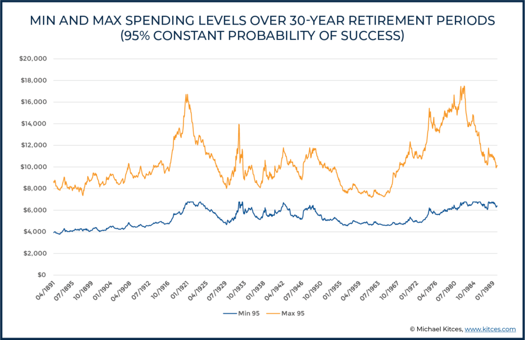
The chart below reports the minimum and maximum levels of real (i.e., inflation-adjusted) spending across the full 30-year time horizons beginning at each date indicated.
Recall that in all of the scenarios above, monthly spending started at $6,769, but, as we see for the period beginning in April of 1891, targeting a constant 95% probability of success led to a minimum real spending level of $3,926 (a 42% reduction) at some point in time during this 30-year period and a maximum real spending level of $8,674 (a 28% increase). In turn, the results not-surprisingly show that during big bull markets – e.g., those who retired in the early 1920s and early 1980s – the maximum spending level may adjust upwards quite dramatically, while remaining more muted in lower return environments.
On the other hand, it’s also notable that in general, the upper level of spending – where it can ratchet up to when markets are good – is actually much more variable than the downside, which varied far less (i.e., the minimum spending to maintain that 95% probability of success was in a fairly narrow band from $4,237 at the 10th percentile to $6,518/month at the 90th percentile for the time periods involved).
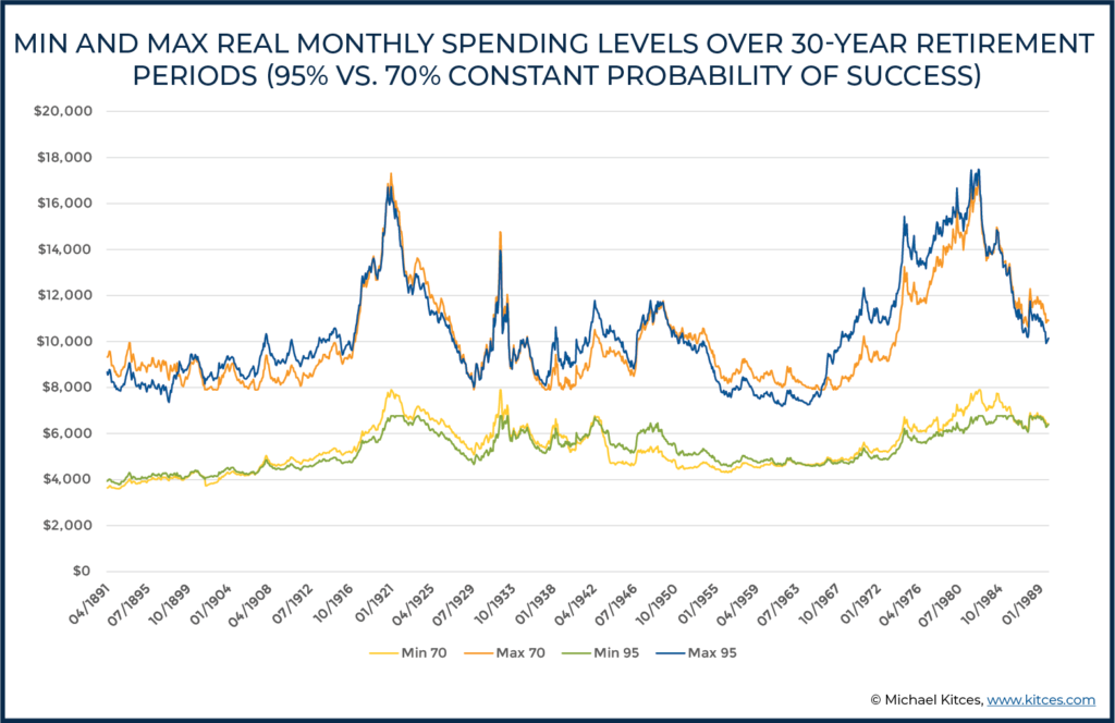
So what happens if a different probability of success level, besides the traditional 95% probability of success target, is introduced to the plan? Instead of targeting a constant 95%, let’s target a lower constant of 70% (with everything else the same). In this case, the lower probability of success means that monthly spending is going to start out a bit higher at $7,898 per month (or $94,777 annually, which is about $1,100/month or almost $13,000/year higher spending from the start), equating to a 5.2% initial withdrawal rate from the portfolio after backing out Hank and Marie’s Social Security benefits.
As Hank and Marie’s 70%-probability-of-success retirement plan then moves through the various time periods in history, making the same adjustments as before to maintain a constant 70% probability of success, the result – for both the constant 70% and constant 95% probability of success levels – are as follows:
When considering the outcomes of maintaining a 70% instead of a 95% probability of success for Hank and Marie, perhaps the most striking outcome is not how different the results are with a lower probability… but, rather, how similar they are! Overall, as long as Hank and Marie’s plan is updated periodically, the minimum and maximum real spending levels experienced really don’t differ much depending on whether you use a 70% or a 95% probability of success! Except by starting at a 70% probability of success, their lifetime spending was able to start $1,100/month (or nearly 16% higher) in the first place!
Which raises the question… what happens at even lower constant probabilities of success?
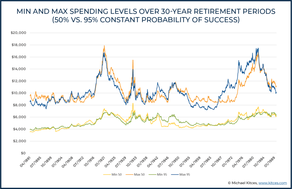
If Hank and Marie become willing to accept an even lower probability of success – given the relatively muted impact that the decrease to 70% actually had – and instead target a constant probability of success of ‘just’ 50%, monthly spending again starts out a bit higher still at $8,462 ($101,547 annually; or about a 6.0% initial withdrawal rate after backing out Social Security).
And as Hank and Marie then move through history, making the same adjustments as before but this time to maintain a constant 50% probability of success, the results compared to the original 95% probability of success are as follows:
What’s again striking, yet again, about these results is how similar they still are from a 95% down to a 50% probability of success. In other words, even if Hank and Marie accept a 50% probability of success, as long as they’re willing to make the adjustments along the way, the minimum and maximum spending levels are still nearly identical!
Of course, the caveat is that for the retiree who starts with a lower probability of success and a higher initial spending level, falling to a ‘similar’ minimum spending level will still reflect a much bigger relative cut in spending from where their retirement started and will be a bigger adjustment to handle.
Yet again, in practice, most of the adjustment is simply to cut the ‘extra’ spending from a higher starting point back to the same minimum spending that may have been necessary had they started more conservatively in the first place. Which means, as long as the retiree is willing to make the adjustments along the way, a higher starting spending level coupled with continuous adjustments doesn’t necessarily cause portfolios to deplete materially faster or to force spending even lower; instead, it simply means spending may have to adjust more quickly in the scenarios where market returns are poor (which then keeps the retiree on track).
We see an example of this looking at the 1940s, where the minimum of the 50% probability of success approach bottoms out significantly lower than the 95% probability of success. And, as noted above, this fall is going to be more dramatic for someone starting out from a higher spending base, even if the ultimate difference in low points is less stark.
For instance, in the period beginning July of 1944, the minimum spending level with a 95% probability of success was about $5,380 per month versus about $4,640 per month with a 50% probability of success. While this difference of roughly 14% is notable on its own, what’s even more notable is that the minimum, with a 95% probability of success, is falling from $6,769 per month to $5,380 per month (a cut of about 21%), but the minimum with a 50% probability of success falls from $8,642 per month to $4,640 per month (a spending decline of about 46%!).
So, while the differences in minimums are less stark, the much larger cuts under the 50% probability of success strategy are likely to feel more wrenching to a client even if they are coming from a higher initial base and the ultimate difference between the two strategies is more muted. Nonetheless, for retirees who are comfortable with adjustments, it may at least make sense to consider lower probabilities of success.
Accordingly, since Hank and Marie from our example are willing to adjust their spending (and especially if they are okay with the idea that, in most cases, the spending cuts they experience will simply trim back the additional spending they wouldn’t have had in the first place with a more conservative starting plan, so why give up the higher spending upfront, and instead wait and see if markets require the cuts instead!?), what if they really push the envelope and try something ‘crazy’… like a constant 20% probability of success!?
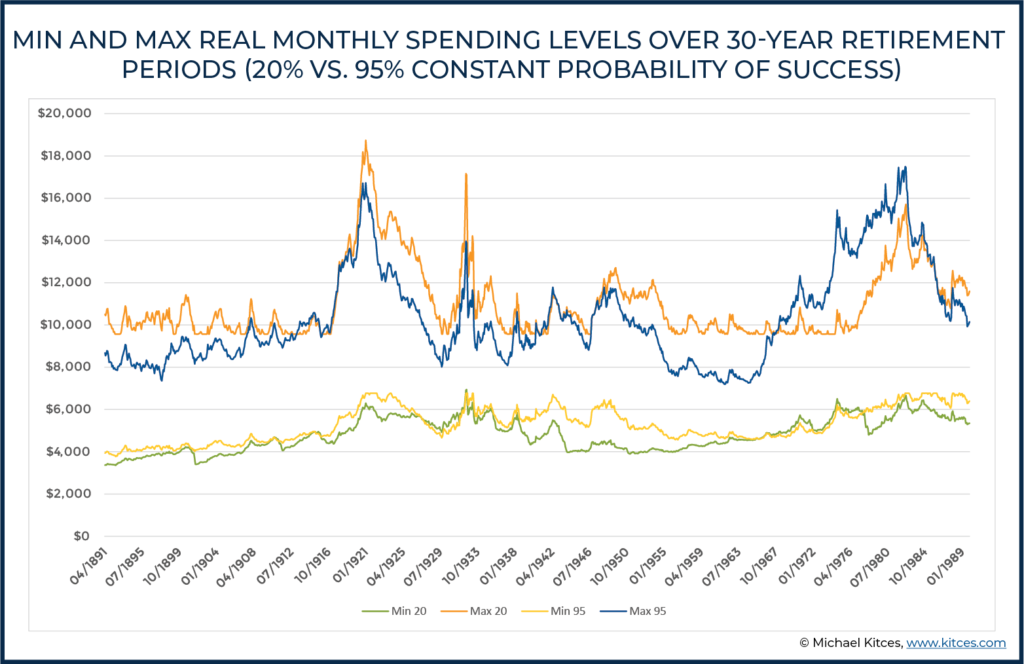
With a 20% probability of success, initial spending will not surprisingly start out even higher at $9,568 per month ($114,815 annually; roughly a 7.3% initial portfolio withdrawal rate after backing out Social Security, and a nearly 40% instead from the starting spending level at a 95% probability of success). The chart below compares the minimum and maximum spending levels for the constant 20% probability of success versus the constant 95% strategy.
When the probability of success is cut down to 20%, there is a bit more of a departure on both the low-end and the high-end from the original 95%-probability-of-success baseline… but likely still nowhere near as devastating as what most retirees (and their advisors) might have expected.
Of course, it’s worth noting that spending declining down to $3,500 per month is still actually the real “$0” here, since we are assuming $3,500 in monthly Social Security income. In other words, if Hank and Marie approach $3,500 in monthly income, that means they’re nearly or completely running out of portfolio income. But, regardless, the difference in minimum and maximum real monthly spending when comparing a 20% probability of success versus a 95% probability of success is not all that different! Especially when recognizing the starting point of the 20%-probability scenario is a spending level that begins 40% (!) higher from the start!
Median Spending Outcomes And Other Cross-Scenario Comparisons
In fact, the reality is that once retirees assume that they will make adjustments along the way, ongoing adjustments tend to cause most retirement paths to converge into a relatively similar range since the whole point of ongoing financial planning, with ongoing adjustments as needed, is to ensure that the plan never deviates too far off track before making a mid-course adjustment to get it on track again!
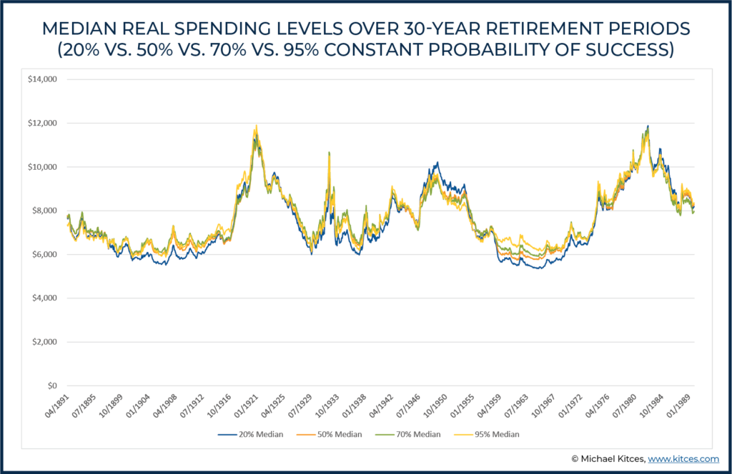
Accordingly, the chart below reports median spending levels across each 30-year time period following the 20%, 50%, 70%, and 95% constant probability of success strategies described above.
As the results reveal, the fact is that, because all plan scenarios – regardless of the probability of success – are rapidly making adjustments in adverse scenarios (so that lower probability of success doesn’t actually result in faster failure, simply faster adjustments), in the end, there is very little difference at all in most outcomes. In almost all cases, median spending actually ends out almost identical regardless of the Monte Carlo probability of success used, with just slightly more spending volatility with a 20% constant probability of success strategy (but nowhere near the level retirees might fear), because the commitment to ongoing adjustments effectively ensures that spending aligns itself.
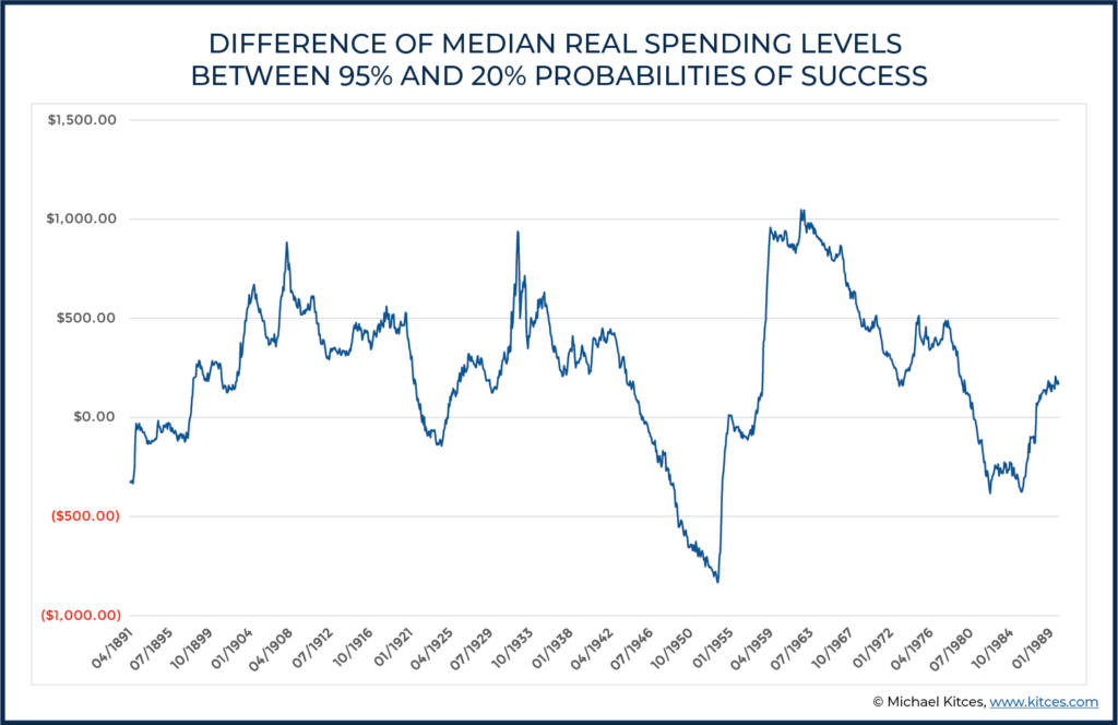
In fact, if we compare the median in the constant 95% probability of success and subtract the median in the 20% probability of success scenario, we can more easily examine the actual differences between these probability outcomes, as shown below:
As the results show, retiree spending between 95% and 20%(!) probabilities of success in practice will rarely differ by more than $1,000 real dollars in either direction (which is barely 15% of the baseline spending of the 95%-probability-of-success retiree in the first place, in a world where retirement research already shows that the typical retiree’s spending declines by far more than this simply with the natural aging process and its impact on spending behaviors!). Simply put, for retirees who are willing to make adjustments, the targeted probability of success really doesn’t make that big of a difference with respect to income! (As again, it’s no longer really a probability of success, because ongoing adjustments always ensure ‘success’; instead, it’s simply the probability that adjustments happen in the first place!)
How Wealth Levels Are Impacted By Different Probabilities Of Success And Spending Adjustments
Of course, the starting probability of success/adjustment clearly does make some difference, though – shading income either slightly higher (lower probability of success) or lower (higher probability of success) – but ultimately the returns experienced in retirement are a much larger factor in determining how much can be spent. While the probability, again, more directly impacts the frequency of the adjustments (and the baseline from which they start).
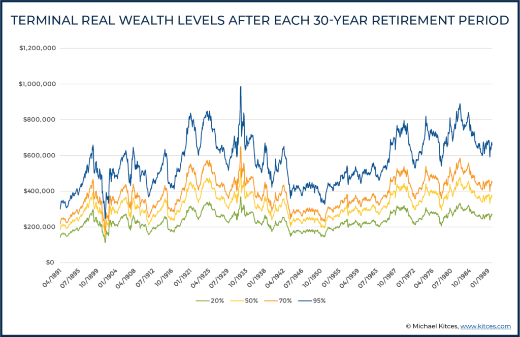
On the other hand, because differing probabilities of success/adjustments can materially change the starting spending levels – which, in favorable markets, simply sustain or rise even further – when multiplied over the duration of the result, they do result in more substantive differences with respect to wealth levels. The chart below reports terminal wealth levels at the end of each 30-year retirement period.
Recall that Hank and Marie had a real legacy goal of $200,000. We see that they never came short of that goal with a 95% or 70% probability of success, fell short of that goal about 2% of the time with a 50% probability of success, and fell short of that goal about 24% of the time (albeit still not by much) with a 20% probability of success.
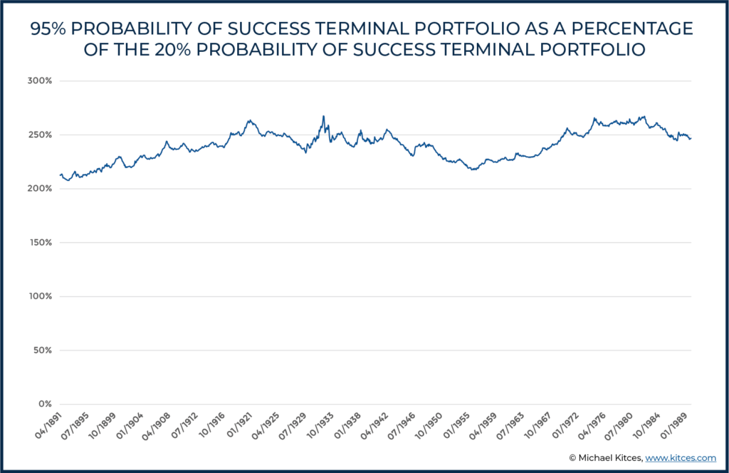
On the other hand, in a world where Hank and Marie had ‘only’ a legacy goal of $200,000, arguably a 95% probability of success that averages almost $600,000 of terminal wealth simply represents a dramatic under-spend for the bulk of their retirement! Especially recognizing that these are inflation-adjusted real dollars; in nominal dollars at a 3% inflation rate, Hank and Marie’s $1,000,000 nest egg finishes with nearly $1.5M instead (whereas their legacy goal was ‘only’ about $500,000 in nominal dollars), thanks to the extraordinary portfolio upside that can occur with conservative retirement spending paths. In fact, as the chart below indicates, the 95% constant probability of success strategy leads to terminal wealth levels that range from about 200% to 260% of the size of the 20% probability of success strategy.
Or stated more simply, the 95%-probability goal, even with continuous spending adjustments, still results in Hank and Marie leaving nearly 3X their legacy goal behind that could have been spent… while the 20%-probability goal, with its more constant adjustments, actually gets them closest to their legacy goal (and does so by allowing them to enjoy more of their money in the earlier years of retirement, without resulting in ruin or the disastrous outcomes that many advisors might anticipate).
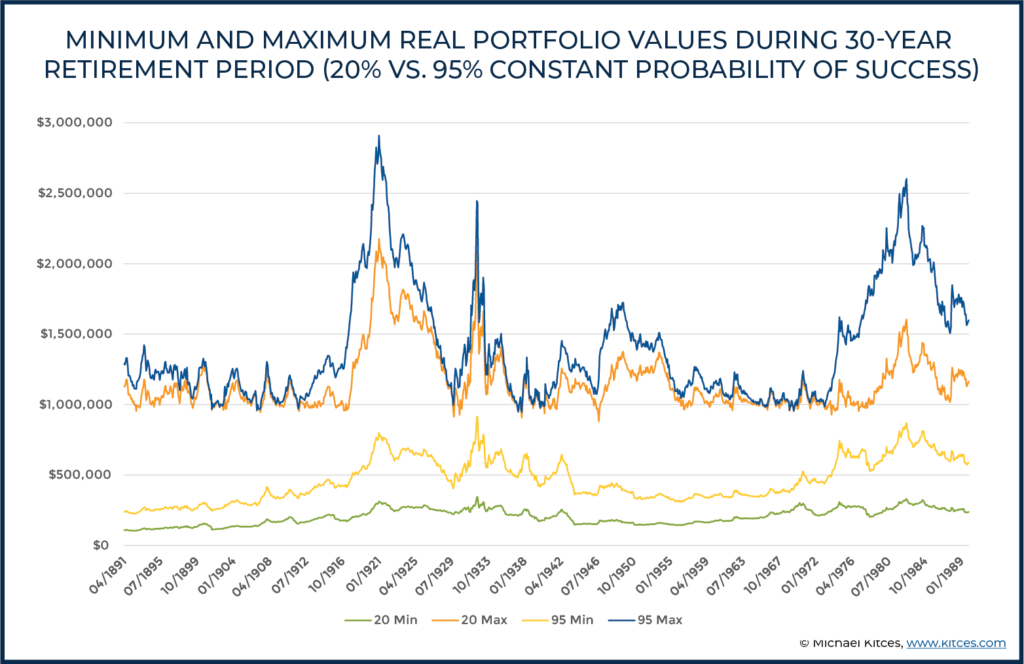
Furthermore, if we look at minimum and maximum real portfolio values attained at any point during retirement (rather than just terminal values), we again see surprisingly little difference between using a constant low probability of success (20%) and a higher probability of success (95%), although we do see more of a difference than we did with spending.
In essence, a lower probability of success does result in “lower highs and lower lows” when it comes to wealth… but does so at the ‘cost’ of higher retirement spending (in the early years before it adjusts down in bad scenarios, or simply sustained higher spending in the ‘good’ bull market scenarios). Which for many retirees is the exact income-vs-legacy trade-off they want to make to enjoy their retirement savings in retirement!
More generally, what these results suggest is that for clients who are willing to make adjustments along the way, the probability of success level chosen is really more a reflection of preferences between income and legacy, than it is a metric for assessing the risk of running out of money.
As again, while the impact on spending levels is very small across a wide range of success probabilities (see earlier chart, “Median Real Spending Levels Over 30-Year Retirement Periods”), the impact on legacy is more significant across the same range of success probabilities (see earlier chart, “Terminal Real Wealth Levels After Each 30-Year Retirement Period”). All else being equal, then, clients who value income more than legacy might want to consider using lower probabilities of success that would allow for higher levels of spending, and for those more concerned about the legacy they leave, a constant 50% probability of success (or even 20%!) is not disastrous.
Other Considerations When Selecting A Monte Carlo Probability Of Success/Adjustment
If planning to a constant probability of success is more a trade-off between income and legacy, then the way we think about the probability of success as advisors is probably due for some change. Most modeling of retirement income strategies (e.g., the safe withdrawal rate) is done with either static planning assumptions or assumptions that suggest some clients will charge forward blindly and keep spending at a potentially disastrous level and deplete a portfolio rather than ever meet with their advisor and make the necessary mid-course adjustments to stay on track.
However, in reality, for clients that are receiving ongoing advice and are able to adjust spending along the way, there’s little risk they would actually ever run out of money, at least assuming that they can and are willing to make the necessary reductions in spending in a subset of adverse (e.g., bear market) scenarios. For our hypothetical couple above, Social Security provided a ‘floor’ of $3,500 in monthly income. How close that floor gets to covering their truly essential expenses is likely an important factor in thinking about what probability of success to use.
For instance, if Hank and Marie are confident that they could make adjustments needed to live off of $3,500 per month and really don’t care to leave more than their $200,000 real legacy, then perhaps a 50% probability of success strikes a good balance between ensuring that they’ll meet their legacy goal without leaving too much income on the table.
By contrast, if Hank and Marie strongly felt that higher spending is a fun ‘splurge’, but dipping below $5,000 per month in income would significantly reduce their quality of life, then perhaps planning to a 70%, 95%, or other higher probability of success would provide better assurance of meeting their monthly income needs.
That said, it is also worth acknowledging that in the retirement periods with the worst sequences of returns, the floor was pretty much the same whether they planned to a 20% or a 95% probability of success. As a result, it may be the case that the client needs to be informed that, despite their strong desire not to go below $5,000 per month in income, there’s some real risk of that happening no matter what probability of success level is used… and that starting with a higher spending level and a lower probability of success doesn’t actually make that adverse outcome worse (i.e., the floor is still the floor), but simply a bit more likely (with a trade-off that in good scenarios it just permits more spending along the way).
Additionally, if a client does have a strong preference for a baseline level of spending, then it may also be a case where using annuity products to build a stronger base of guaranteed income is a prudent avenue to explore.
Another consideration for advisors (and clients) is to consider how generally feasible it may be to make spending changes if/when needed. A benefit of using a lower probability of success is the higher initial spending amount it provides. However, it may be the case that starting with a high spending level and then cutting it down over time would prove more difficult, at least for some clients, than starting at a lower spending level to begin with. In other words, it may be harder to spend more and have to cut the retirement lifestyle back, than simply never introducing the higher lifestyle spending by choosing a higher probability and more conservative initial spending in the first place.
After all, in the scenarios for Hank and Marie considered earlier, initial spending ranged from $6,769 (95% probability of success) to $9,568 (20% probability of success) per month. On the one hand, starting at a higher monthly income means that even the first $2,800 in ‘cuts’ are not really reductions relative to the alternative strategy, at it would simply trim the $9,568/month spending back to the $6,769/month baseline being considered in the first place. On the other hand, if monthly spending does eventually need to be cut to $6,000, the reduction from $6,769 down to $6,000 may hurt less than the reduction from having started at $9,568.
However, particularly when thinking about the many Americans who may not be in as strong of a position as they would ideally like to be in their future retirement, another takeaway here is that perhaps they don’t need to be overly stressed out if their plan is showing 50% (or less) probability of success!
Consider these two possible ways of presenting a 50% probability of success result to clients who are hoping to retire today:
- Scenario 1: “Mr. and Mrs. Client, after running your plan, we found that you have a 50% probability of success, implying a 50% chance that your retirement will fail. As you can see on the confidence dial, that is outside of our comfort range, and you may want to consider spending less or delaying retirement until we can increase that probability of success and reduce the risk of failure.”
- Scenario 2: “Mr. and Mrs. Client, your plan is coming in at 50% probability of adjustment. While that means there is a decent chance you may need to make some spending cuts in the future, if you are willing to make those cuts if needed, then you can go ahead and retire today. Alternatively, if you’d like to reduce the risk of needing to make some adjustments in retirement, you could delay the start of your retirement instead, if you prefer.”
These scenarios work with the same client results and the same probability outcome, but illustrate two very different ways of framing them. One will likely cause a lot more client anxiety than the other, but neither is wrong, per se. It is true that spending less or working longer will increase the probability of success. However, at the same time, it is also true that we are only talking about adjustment (not failure) for clients in ongoing advice relationships who engage in ongoing monitoring and make ongoing adjustments. And we haven’t even begun to address the magnitude of adjustment that is needed to keep the plan on track (which in some cases is itself fairly minor).
Unfortunately, addressing this additional dimension of retirement preparedness is really hard to do with most technology tools available today, as modern financial planning software is heavily focused solely on probability of success, and the type of dynamic spending adjustments modeled above simply is not possible to model. While some newer tools are developing that functionality, the simple reality is that most don’t give advisors the information needed to begin exploring these different considerations and trade-offs with clients and reflect what happens when clients can and do work with their advisors to make retirement spending adjustments as needed on an ongoing basis.
The key point, though, is simply that the decision of choosing what probability of success to use is not as simple as being able to apply to a one-size-fits-all rule or a natural tilt towards being ‘conservative’ for the sake of not having retiring clients run out of money on the advisor’s watch. For those retirees who are willing and able to make needed adjustments along the way, a 50% (or lower!) probability of success may provide a better result than most advisors (and clients) realize!
Disclosure: Derek Tharp is a Senior Advisor at Income Lab, which provided some coding support for the Matlab models used in the examples included in this article.


