Executive Summary
One of the questions retirees often have is how much they can afford to spend each year over the course of their retirement without depleting their portfolio during their lifetimes, and financial advisors have many tools to aid in this discussion. One classic technique is the use of withdrawal rates; based on asset allocation and historical return data, advisors can calculate a safe annual portfolio withdrawal rate that retirees can use to guide their spending throughout their retirement. However, this approach does not account for the investment returns the clients actually experience in their retirement; for example, the safe withdrawal rate could increase over time if the client experiences strong investment returns in their first few years of retirement.
To solve this problem, advisors can use withdrawal-rate guardrails, which are guidelines to increase or decrease spending when portfolio withdrawal rates reach certain levels. For example, if an initial 4% withdrawal rate calls for $5,000 in monthly spending, the spending amount could be adjusted higher if it reaches 2% of the portfolio value or lower if it hits 6%. Yet, withdrawal-rate guardrails can be flawed because the relatively steady withdrawal rate patterns used do not necessarily align with how retirees actually pull distributions from a portfolio in retirement.
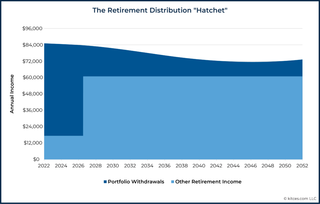
In reality, what is more commonly seen is a “retirement distribution hatchet” in which the initial retirement distribution rates from a portfolio are highest early in retirement, then significantly decline when deferred Social Security is claimed (as late as age 70), and falling further yet because of the tendency for retirees’ spending to decline in real dollars as they move through retirement. A dynamic portfolio withdrawal strategy should also consider other sources of income in retirement (e.g., pensions, rental properties, part-time jobs, house downsizing, and inheritances) that can impact the size of needed portfolio withdrawals to cover spending requirements.
To compensate for this issue, advisors can consider using holistic risk-based guardrails, which reflect current longevity expectations, expected future cash flows, expected future (real) income changes, and other factors. Probability of success via traditional Monte Carlo analysis can serve as the risk metric to guide the implementation of risk-based guardrails. There is a risk of causing anxiety for clients if the risk is presented in terms of the success or failure of their plan as a whole, but advisors can instead use the language of income risk, which may be less stress-inducing. For example, an advisor could explain that if risk increases (e.g., if investment returns are weak), downward adjustments to spending will be needed; alternatively, if risk declines (e.g., because the client has reached an advanced age with a strong portfolio) spending can be safely increased.
Ultimately, the key point is that a risk-based guardrails model can provide clients with a more accurate picture of how much they can sustainably spend than can models based on static withdrawal rates or withdrawal-rate guardrails. While risk-based guardrails can be less efficient to calculate manually than withdrawal-rate guardrails because of the many factors considered in the risk-based model, when properly assisted by technology, risk-based guardrails can be implemented and maintained as efficiently as withdrawal-rate guardrails. And, given how different the retirement distribution hatchet is from the distribution patterns assumed by withdrawal-rate guardrails, the movement from withdrawal-rate guardrails to risk-based guardrails represents a significant improvement in planning quality for retirees!
Withdrawal-rate guardrails – i.e., guidelines to increase or decrease spending when portfolio withdrawal rates reach certain levels – have obvious utility when it comes to retirement income research and testing dynamics related to how much retirees can spend in retirement. Frameworks that rely on such guardrails, like the Guyton-Klinger model, have even provided new insight into how retirees can dynamically adjust spending in retirement. In practice, however, withdrawal-rate guardrails have some serious flaws. Most importantly, such frameworks describe withdrawal rate patterns that don’t align with the reality of how retirees actually pull distributions from a portfolio in retirement.
Rather than the relatively constant withdrawal rate through time assumed by such guardrail models, withdrawal rates for many retirees decrease significantly over the first 5-10 years of retirement and then show a more gradual decline in subsequent years. The primary driver of this is the deferral of claiming Social Security, which, once claimed, drastically reduces the income needed from a portfolio.
A secondary driver of this withdrawal rate reduction over time is the natural decline in overall real spending that is observed among retirees – as described through research such as David Blanchett’s retirement spending smile. Even though spending in some categories tends to go up with time (e.g., healthcare), general spending tends to decline in real dollars for some households as they move through retirement. This general decline in spending further alleviates the stress that would be placed on a portfolio relative to what is assumed by withdrawal-rate guardrails.
In reality, what we tend to see is a retirement distribution "hatchet”, in which the initial retirement distribution rates from a portfolio are highest early in retirement, then significantly decline when deferred Social Security is claimed (as late as age 70) and decline further as spending declines according to a retirement spending smile.
Why Withdrawal Rates Are Poor Candidates To Use As Income Guardrails
Although withdrawal rates may not be ideal candidates to use for income guardrails, it is still important to understand how they work and the role they’ve had historically in establishing guardrail strategies. Withdrawal rates are calculated by dividing the dollar amount of portfolio withdrawals by the portfolio balance. For example, a retiree might begin retirement taking $40,000/year from a $1 million portfolio for a 4% annual withdrawal rate. If, sometime later (and despite ongoing withdrawals), the portfolio grows to $1.2 million, the withdrawal rate is $40,000 ÷ $1,200,000 = 3.33%. If, instead, the portfolio balance hits $800,000, the withdrawal rate is $40,000 ÷ $800,000 = 5%. Income in dollar terms has stayed the same, but the withdrawal rate has changed.
Many approaches to dynamic retirement income planning that have been explored in research studies suggest that income should be changed if withdrawal rates hit certain pre-set ‘guardrails’. For example, we might manage retirement income by adjusting withdrawals with the following rules.
Withdrawal-Rate Guardrail Example
- Begin with a 5% withdrawal rate
- Increase income if the withdrawal rate goes down to 3%
- Decrease income if the withdrawal rate rises to 6%
The intuition behind withdrawal-rate-based income guardrails is that the withdrawal rate tells us something about the risk of the current income level. The chances that $40,000 annual withdrawals could, over time, deplete an $800,000 portfolio are clearly higher (as are the associated 5% withdrawal rates) than the chances that the same withdrawals could deplete a $1 million (with a lower 4% withdrawal rate) or $1.2 million portfolio (an even lower 3.33% withdrawal rate). Therefore, it may seem reasonable to base our guardrails on withdrawal rates.
But, though this reasoning may seem compelling for simple examples, withdrawal rates are actually poor candidates for income adjustment guardrails. They fail to account for both changes in risk over time as retirees age (e.g., an 8% withdrawal rate is riskier at 65 than it is at 95) and the unique cash flows (and spending habits) anticipated within many households’ income plans (e.g., a retiree that knows they want to fund future weddings for grandchildren).
Longevity Matters
Withdrawal-rate guardrails like those shown above are static: the same values (5%, 3%, and 6% in the example above) would be applied through time as a plan plays out. But the risk of a given withdrawal rate is not the same for all ages and levels of health. The risk of a 4% withdrawal rate is not the same at age 65 as it is at 80; as while a person with a 30-year planning horizon accepts a certain risk by taking $40,000/year from a $1 million portfolio, a person with a 15-year planning horizon takes a much lower risk with the same behavior. This fact makes it impractical to plan for retirement income adjustments with one small static set of withdrawal-rate guardrails.
Notably, some withdrawal-rate guardrails approaches have attempted to account for this. For instance, the Guyton-Klinger model relaxes the guardrails rules in the final 15 years of a projected retirement period. However, this results in a relatively crude breakpoint when the reality is that guardrail risk follows a smoother glidepath through all of retirement.
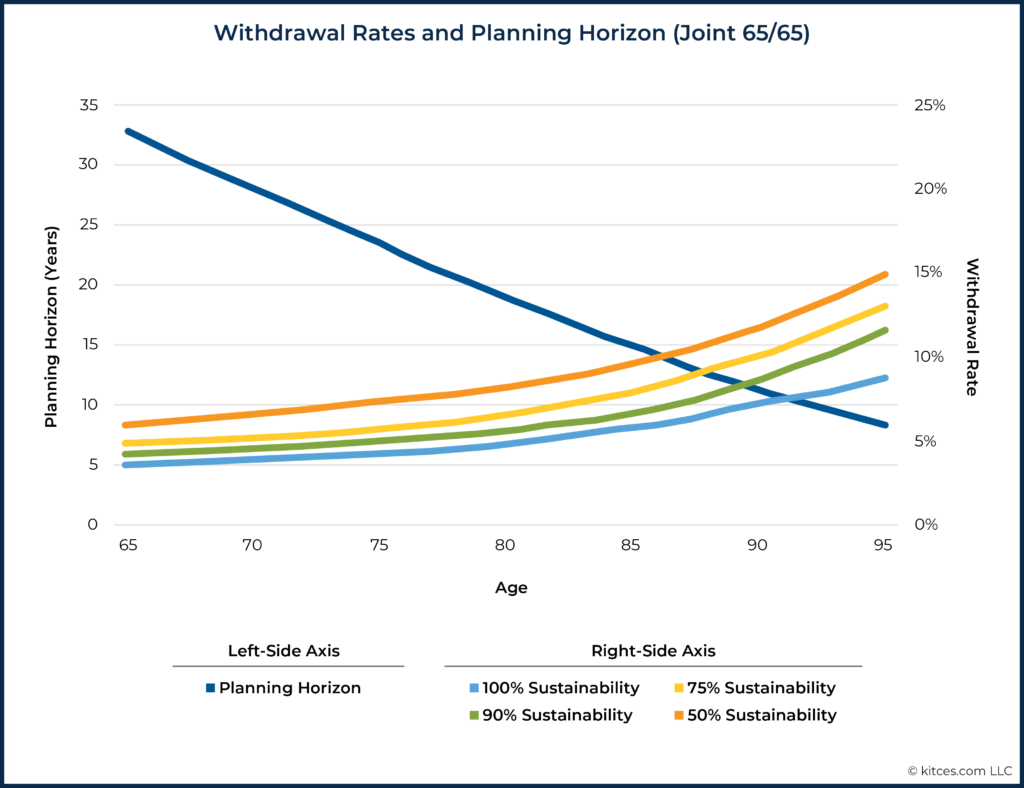
To explore this further, let’s define “longevity risk” as the chance of living beyond a given time horizon. For example, let’s consider Mary and John, who are a married couple and are both 65 years old. If there is a 30% chance that at least one spouse will live beyond 32.7 years, we’d say that the couple has a 30% longevity risk with a 32.7-year planning horizon. But as Mary and John age, the planning horizon that has a 30% risk level would slowly decrease. Keeping longevity risk constant at 30%, their estimated joint planning horizon would be 23.3 years at age 75. By age 85, it would be 14.8 years. (These estimates are based on the Society of Actuaries RP-2014 mortality tables with MP-2017 improvements. An advisor could, of course, choose to base plan length on a different level of longevity risk.)
As people age, planning horizons shrink as shown by the dark blue line in the graph below that slopes down and to the right (left axis). And, as planning horizons shrink, higher withdrawal rates can be sustained, as shown by the rising withdrawal rate lines (right axis) and as the risk of any given withdrawal rate decreases.
The chart below shows estimates of the withdrawal rate that Mary and John could take from a 60/40 stock/bond portfolio at various levels of “sustainability”, which, in this context, is the estimated chance that a given withdrawal rate would survive to the end of or past the corresponding planning horizon.
Given how the risk of withdrawal rates changes as we age, it seems clear that withdrawal-rate guardrails would have to change as well. We would not want to apply the same withdrawal-rate guardrails that we establish at age 65 once we have reached age 75 or 85.
Let’s assume that Mary and John were following the withdrawal-rate-guardrails strategy defined above, with a static 3% withdrawal-rate income-increase guardrail and 6% income-decrease guardrail. They begin retirement at age 65 with a 5% withdrawal rate and, at age 75, find that they have reached a 6.1% withdrawal rate. The guardrail rules would counsel a reduction in income. But, as the chart above illustrates, at this point, a 6.1% withdrawal rate would have an estimated sustainability that is higher than the couple’s original 5% withdrawal rate! In other words, it might actually be more prudent for the couple to increase their income at this point than to decrease it.
This example demonstrates how using static withdrawal-rate guardrails may put us in danger of having not only the wrong guardrail values but of doing the opposite of what is called for when a guardrail is reached!
Of course, the chart above only applies to one age/sex combination (male/female, both age 65). Other combinations would have other values, and if one spouse were to pass away, the surviving spouse would then plan with single-life data, which would have its own set of planning horizons and corresponding withdrawal rates.
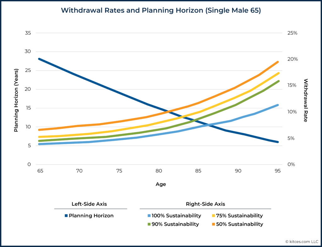
For example, keeping longevity risk the same (30%), a single 65-year-old male would have the following planning horizons and withdrawal rates through age 95.
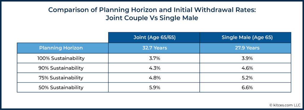
Comparing the charts for a joint couple and a single male (all age 65), there are obvious differences. The single male has a lower planning horizon and higher withdrawal rates at all sustainability levels.
The particularities of age, sex, and single/joint life expectancy make setting general rule-of-thumb withdrawal-rate guardrails impractical. Furthermore, these withdrawal rates correspond only to a particular asset allocation (60/40 stock/bond), fee level (0% in this example), and legacy goal ($0 here). Changes to these assumptions would yield different results, and therefore different guardrails. And, even if it were possible to establish guardrails for each combination of these parameters, the guardrails would have to change over time to account for changes in longevity expectations over time.
Spending Changes Matter
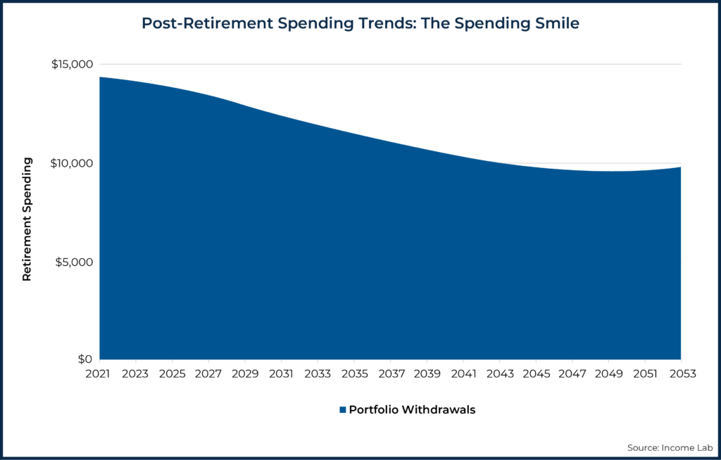
The longevity and withdrawal-rate estimates above assume that retirees will need to maintain their purchasing power through all years of retirement. If a couple is spending $10,000/month in 2021 at age 65, this assumes they will also need $10,000/month, in today’s dollars, in 2041 at age 85. At a 2.5% average annual inflation rate, they would be spending $16,386/month in future dollars by that point.
But research on spending patterns in retirement does not support this assumption of flat, inflation-adjusted spending. Instead, it appears the retirees often spend the most during the early stages of retirement (with, in some cases, year-over-year increases in inflation-adjusted spending), followed by a long period of decreases in inflation-adjusted spending.
Toward the end of life, some may increase their inflation-adjusted spending for medical reasons, although, notably, in David Blanchett’s famous retirement spending “smile”, spending rates were found to generally decrease even as the rate of change was decreasing at a decreasing rate (i.e., it is the first derivative that creates the “smile” in the retirement spending smile and not the spending pattern itself).
A hypothetical spending pattern that matches the description above (with a slight increase in total spending later in life), could look something like this:
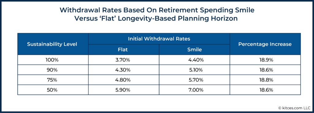
Planning for future spending that changes realistically with age can go a long way toward providing more income to retirees when they need it without depriving them of the income they need later in life. For example, Mary and John, our 65-year-old couple, would have initial withdrawal rates that are nearly 20% higher at various sustainability levels if they planned using the retirement spending smile, in comparison to the initial withdrawal rates determined when assuming flat inflation-adjusted spending.
But, while planning with the retirement spending smile is both supported by research and advantageous at the beginning of retirement, it would make withdrawal-rate guardrails even more difficult to work with. We might start retirement spending $57,000/year from a $1 million portfolio, but plan for spending to go down to $40,000, in real terms, by age 90. These withdrawals are not consistent, so they cannot be managed dynamically using a single set of static withdrawal-rate guardrails.
The clearest problem for withdrawal-rate guardrails in the face of planned changes in retirement income is that we now have to distinguish between planned changes in income and unplanned changes due to unexpectedly low or high portfolio returns. In other words, we would have to distinguish between changes in withdrawal rate that are expected as we follow the retirement smile and those that are not.
For example, imagine John and Mary are using the retirement smile and set the following withdrawal-rate guardrails for use with their $1 million portfolio:
Withdrawal-Rate Guardrail Example (Adjusted for Smile)
- Begin with a 5.7% withdrawal rate
- Increase income if the withdrawal rate goes down to 4%
- Decrease income if the withdrawal rate rises to 7%
Following the smile-adjusted withdrawal-rate guardrails, they plan to withdraw 5.7% (beginning withdrawal rate) x $1 million (portfolio balance) = $57,000/year at the beginning of retirement but $52,000/year ten years into the plan (roughly a 1% annual reduction in real spending). If their portfolio reaches $1.4 million in ten years, they will have reached the $57,000 (withdrawal) ÷ $1.4 million = 4%-withdrawal-rate guardrail. But should this trigger a spending increase, or should Mary and John stick to their originally planned decrease to $52,000/year, representing a 3.7% withdrawal rate? It’s hard to say.
In this instance, their withdrawal rate went down through a combination of a (planned) 10% reduction in dollar withdrawals and a 40% (unplanned) increase in their portfolio. To better account for planned spending changes, our withdrawal-rate guardrails would not only have to take into account current withdrawals and account balances, but would also have to adjust over time for past and future planned changes in real withdrawals. This situation does not lend itself to a simple set of static withdrawal-rate-based guardrails.
Cash Flows Matter
So far, we’ve been treating retirement income as entirely funded by portfolio withdrawals. But for most people, this is not realistic. Income from Social Security, pensions, rental properties, part-time jobs, house downsizing, and inheritances are only a few of the factors that can make the actual cash flow picture for most families quite complex.
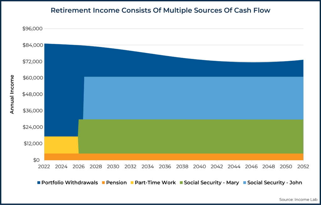
For example, let’s give our 65-year-old couple, Mary and John, two Social Security income streams, income from part-time work for five years, and a pension.
Initially, only portfolio withdrawals, part-time work, and the pension will be used to fund retirement income, leading to an initial 6.7% withdrawal rate. As Mary and John’s Social Security kick in, annual planned withdrawals are down to approximately $55,000 in 2026 and $24,000 in 2027, respectively. Due to the retirement smile, withdrawals continue to decrease in real terms, going as low as $10,500/year when Mary and John are both age 90 in 2046. The portfolio withdrawals, on their own, are anything but flat as a dollar amount or as a percentage of total planned income.
With a complex stew of income sources and retirement spending smile considerations, there is simply no chance that we could define a clear set of relatively stable withdrawal-rate guardrails. Instead, we would need a different set of guardrails for each point in the plan. This would make client communication using withdrawal rate guardrails very difficult.
Notably, once we account for unique client-specific cash flows, not everyone’s retirement spending will have a ‘hatchet’ shape to it. Just as some retirees may not follow a retirement spending smile and may actually spend at a constant inflation-adjusted rate, or possibly even increase spending over time, not every retiree’s spending shape will align with the retirement distribution hatchet. Nonetheless, the general tendency for the hatchet to emerge (via the combined forces of both delayed Social Security and declining spending over time) is sufficient to generate concern regarding the application of withdrawal-rate guardrails as is most commonly done today.
Holistic Risk-Based Guardrails: An Alternative To Withdrawal-Rate Guardrails
Recall that withdrawal-rate guardrails had the apparent advantage of being intuitive: they seemed to correspond to differences in income risk. But even if we could produce a complex set of tables that told us when withdrawal rates should trigger income changes at each point in time for all age/sex combinations, longevity risk levels, investment mixes, fee levels, income paths, and non-portfolio income (a set of tables that would be infinitely large), we would have lost the intuitive, natural feel of our initial static withdrawal-rate guardrails and the simplicity of communicating these guardrails to clients. Since withdrawal-rate guardrails are impractical and even flawed in the ways we just saw, we might search for income adjustment guardrails that return us to the same place: guardrails that correspond directly and intuitively to income risk.
In fact, such guardrails are easy to find: instead of stating guardrails in terms of withdrawal rates, we can simply state them in terms of estimated overall risk. The income-risk measure we use for these guardrails should be holistic, meaning it should reflect current longevity expectations, expected future cash flows, expected future (real) income changes, and so on.
Probability of success from a Monte Carlo simulation would be one such candidate for a holistic measure of risk to drive guardrails. However, there are a number of known issues with framing results around probability of success, so considering alternative metrics may be worthwhile.
When working with dynamic income planning, it can be helpful to avoid success and failure language, so as to reduce the chances of misunderstanding and heightened client anxiety. With this in mind, we could define overall income risk as the chance that a given income plan is not sustainable through the plan horizon, and so could require a downward adjustment. This holistic measure can be re-estimated as often as we like to reflect the facts on the ground and any updated assumptions. But even with all of these complexities, such guardrails could be stated very simply, as illustrated in the following example:
Holistic Income-Risk-Guardrail Example
- Target an initial income risk of 20%
- Increase income by X if the risk of the current income plan goes down to 0%
- Decrease income by Y if the risk of the current income plan rises to 60%
Here X and Y could be almost anything: a percentage change, a dollar change, a change in risk level, or a movement toward another risk level (e.g., “return to an income with the target risk level of 20%”).
We can use the same risk concept over years and decades, even as the things that lead to those risk levels change. Additionally, this approach has the advantage of keeping conversations with clients at the right level of abstraction. Rather than discussing withdrawal rates, mortality curves, and other obscure or difficult-to-understand concepts, we are simply discussing overall, holistic risk. We can fold as much complexity and sophistication as we want into the model that produces these risk estimates while continuing to keep discussions at a higher level. Income change guardrails can be communicated in plain language without the need to specify withdrawal rates: If risk goes up sufficiently, we’ll tighten our belts. If it goes down sufficiently, we’ll feel free to spend a bit more.
Implementing Risk-Based Guardrails In Practice
One advantage of Guyton-Klinger and similar withdrawal-rate guardrail methodologies is the simplicity of a defined set of rules that are easy to check. This advantage should not be overlooked, as simple heuristics can sometimes be the best available course of action – particularly in the context of do-it-yourself retirees who may lack the specialized knowledge and access to technology that makes more holistic risk-based approaches feasible.
However, if the goal is to develop the best set of guardrails possible that balances both upward and downward adjustment throughout retirement, then the retirement distribution hatchet should not be ignored.
Particularly for advisors serving in a fiduciary capacity to help clients navigate retirement, the ability to develop specialized knowledge and leverage technology to implement a more sophisticated guardrails strategy should not be overlooked.
Fortunately, there are a number of ways to implement risk-based guardrails in practice. As previously mentioned, probability of success via traditional Monte Carlo analysis could serve as the risk metric to guide the implementation of risk-based guardrails. While the process can be a bit cumbersome with traditional Monte Carlo software, it can still be done… guardrails have been successfully emerging as an efficient way for advisors to do financial planning for clients while also presenting information in a more valuable format.
Essentially, to implement probability-of-success-driven guardrails, advisors would need to solve for an initial target probability of success (e.g., 90%), and then decide on upper and lower guardrails that would warrant spending changes (e.g., increase spending at 99% probability of success; decrease spending at 70% probability of success). The next step would be to determine the portfolio values that would result in hitting those guardrails today so that the guardrails can be expressed to clients in dollars (versus a more abstract probability-of-success percentage), which also serves to capture the communication advantages of guardrails. Finally, advisors would solve for the spending levels that would bring the probability of success back to the target at these higher/lower guardrails (so that the adjustment at the upper/lower guardrails can be communicated to clients as actual dollar amounts, to help manage expectations).
The process of setting guardrails with Monte Carlo analyses would involve extensive trial-and-error or ‘guess-and-check’ work, and so is a bit cumbersome. Ideally, technology should be able to automate this guardrails process for advisors so that the advantages of risk-based guardrails can be captured without bringing in the disadvantages of withdrawal-rate guardrails. And, indeed, some tools have begun to provide that automation.
Furthermore, ideal technology solutions should be able to track a plan’s progress over time. Particularly if account values don’t need to be updated manually, then risk-based guardrails should be able to monitor progress over time and alert advisors when a guardrail is near or approaching.
While risk-based guardrails can be less efficient to calculate manually than withdrawal-rate guardrails (since withdrawal-rate guardrails have the advantage of disregarding the retirement distribution hatchet), when properly assisted by technology, risk-based guardrails can be implemented and maintained as efficiently as withdrawal-rate guardrails. As such, risk-based guardrails can be used in conjunction with a surge meeting process to deliver greater planning efficiency.
In an ideal world, for a niched advisor working with retirees, guardrails could be monitored in the background, and guardrails reports (ideally as a one-page financial plan) could be generated for an entire client base with no more than a click of a button, dramatically reducing the burden of updating client plans in preparation for a surge cycle.
But regardless of whether advisors are using tools specifically designed to help with guardrails implementation or standard Monte Carlo tools that are the norm within the industry, the reality is that risk-based guardrails that account for the retirement distribution hatchet can be implemented. And, given how different the retirement distribution hatchet is from the distribution patterns assumed by withdrawal-rate guardrails, the movement from withdrawal-rate guardrails to risk-based guardrails represents a significant improvement in planning quality for retirees!
Disclosure: Justin Fitzpatrick is Chief Innovation Officer at Income Lab and Derek Tharp is a Senior Advisor at Income Lab. Income Lab was used in calculating the examples included in this article.


