Executive Summary
Given the myriad of products and services available to today’s prospective retirees, there are a lot of choices to consider about which retirement income strategy to pursue, from portfolio-based withdrawal strategies to annuities with income guarantees and more.
Yet as it turns out, what seems like a relatively simple question – which retirement income strategy is the best – is actually remarkably difficult to determine. Because as it turns out, which is “best” depends heavily on how you measure what “best” really means in the first place.
For instance, when evaluating by what produces the most wealth, the best retirement strategy is generally to just not spend very much (and ideally invest for growth along the way, too)! If the goal is to maximize retirement spending, then the “best” strategy is to invest as aggressively as possible in order to maximize the portfolio growth that will substantiate that spending. Yet portfolios with maximal growth can also produce the greatest catastrophes, which means a risk-averse retiree may not want that approach, even if it would otherwise have increased retirement spending!
What all of this ultimately means is that in framing different retirement income strategies – and the trade-offs they might entail – it’s important to give serious consideration to the measuring stick that will be used to evaluate the potential retirement outcomes. Because the “best” retirement income strategy may be very different depending on whether you measure based on wealth, spending, probabilities of success, magnitudes of failure, or utility functions that weigh both the upside and downside risks!
Determining How To Measure The 'Best' Retirement Strategy
Imagine for a moment that a 65-year-old couple is trying to decide how much to spend for a 30-year retirement from their $1,000,000 portfolio, and how that portfolio should be invested. The seemingly simple trade-off choices might include:
A) Spend an inflation-adjusting $30,000/year from the portfolio, by putting 90% of it into an immediate annuity and keeping the other 10% in cash reserves
B) Spend an inflation-adjusting $45,000/year from the portfolio, and invest it 50/50 in stocks and bonds
C) Spend an inflation-adjusting $60,000/year from the portfolio, and invest it 100% in stocks
While many advisors might intuitively lean towards one strategy or another as likely to be the “best”, it turns out that accurately assessing which is really the best depends heavily on how the outcome is measured in the first place.
Measuring Retirement Outcomes By Projected Wealth
The first way these three strategies might be assessed – and the most common methodology for the first several decades of financial planning – is to project how wealth would accumulate and compound over the 30-year retirement time horizon.
For instance, the chart below graphs the remaining wealth in the portfolio across each of the three strategies, assuming inflation averages 3%, and that long-term 30-year investment returns are 3% for cash, 5% for (intermediate) bonds, and 10% for stocks. (The immediate annuity is assumed to have a principal refund feature if death occurs before the payments have been recovered, which winds down over time as the payments are made.)
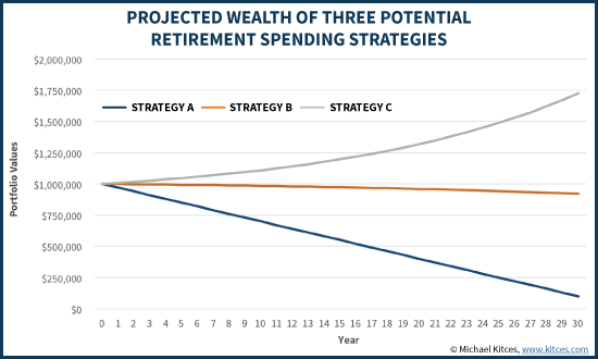
As the chart illustrates, on the basis of this analytical approach – which strategy accumulates the most wealth in the long run – strategy C is the best. Ironically, this is true even though in general, long-term wealth would actually be maximized by spending the least (and allowing the most to compound for future growth), which would have been strategy A. Yet in this case, the long-term compounding return of stocks is so dominant, that strategy C creates the most long-term wealth, even though its growth is slowed by what are also the largest ongoing withdrawals.
Measuring Retirement Outcomes Based On Cumulative Spending
Notwithstanding the fact that strategy C actually turned out to create the most wealth – despite taking the largest withdrawals – in practice, retirees who ultimately want to enjoy retirement should probably not measure outcomes based on final wealth alone. Otherwise, for any two strategies that have similar returns, the “better” one will always be the one with the least spending, which at the logical extreme would mean the “most successful” retirement strategy is the one where the clients never spend a dime of their retirement funds!
An alternative approach would be to look at the cumulative amount of dollars actually spent, which more accurately represents the retiree’s opportunity to actually enjoy the retirement portfolio. In this context, the “best” strategy will not be the one that leaves the most money in the portfolio at the end, but the one that allows the most money to be consumed while the retiree is alive.
In this case, evaluating outcomes based on cumulative spending once again supports strategy C as the “best”. As shown below, strategy C produces by far the largest amount of cumulative retirement income spending, in addition to the fact that it also produces the greatest wealth accumulation over time (as shown earlier), thanks again to the long-term compounding return of equities.
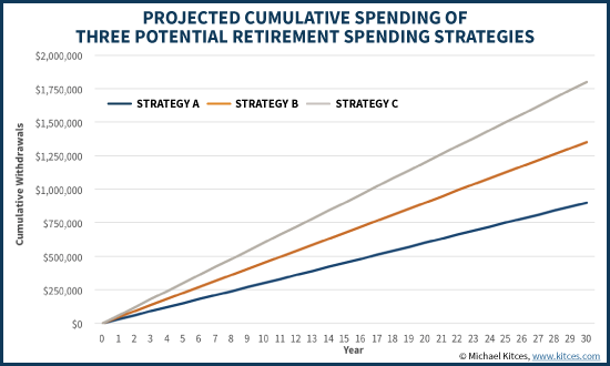
Of course, the caveat to this methodology is that it doesn’t just show projected wealth and cumulative spending, per se. It shows the projected levels of wealth and spending if average returns are earned. Moreover, it’s based on having returns average out to their long-term target with no volatility along the way.
Yet a zero-volatility growth-in-a-straight line projection is not reflective of the real world. When the dynamics of real-world are considered – i.e., the “best” strategy is evaluated not based on linear projections but a different measuring stick – suddenly the optimal approach changes.
Measuring Retirement Outcomes Based On Probability Of Success
Over the past 15 years, as computing power has continued to grow exponentially, it’s no longer necessary to project the financial outcome of a strategy by just measuring the economic impact based on average returns. Instead, we can now measure economic outcomes by modeling thousands of possible scenarios, each with randomized returns (based on the probability that they will occur), and instead quantify how often the results are “successful” (i.e., have money left at the end) or are not (i.e., run out of money before the end of the time horizon). This approach is commonly known as Monte Carlo retirement analysis.
When using this different methodology to quantify retirement outcomes, though, the relative benefits of each strategy begin to look very different as well. For instance, the chart below shows the Monte Carlo outcomes of our three retirement strategies, including the range of possible outcomes based on a 95% confidence interval (long-term returns that are plus-or-minus two standard deviations).
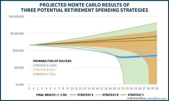
When measured earlier based on (median) final wealth and cumulative spending dollars, the “best” scenario was the all-stock strategy C and the worst was the immediate-annuity-based strategy A (with the latter coming in last in terms of both spending and wealth accumulation). Yet now when we observe the range of results, Strategy C has the best average but also includes the worst failures (including financial ruin as early as the 22nd year of retirement), while Strategy A has an extremely narrow range of outcomes that are “mostly” well below the average of Strategy A… but none of them are failures!
In other words, based upon probabilities of success instead, annuity-based strategy A is now the “best” – a 100% probability of success, with no projected failures (presuming the annuity company is secure in the first place) – and strategy C is the worst (the lowest probability of success and highest frequency of depletions/failures). The entire sequence of which retirement strategies are “best” changes completely when using a different measuring stick, as the “best” for accumulating wealth and spending on average is the all-stock portfolio but the “best” for avoiding any risk of depletion is to spend less and annuitize assets to secure that spending goal!
Measuring Retirement Outcomes Based On Magnitudes Of Failure And Adjustment
The charts in the prior section – based on probabilities of success – showed that strategy A was “best” and superior to both strategy B and strategy C. However, a more nuanced look reveals that just choosing the plan with the highest probability of success (and lowest probability of failure) may not be the ideal approach, either.
After all, the probabilistic “superiority” of strategy A (the $30,000/year annuity approach) over strategy B (spending $45,000/year from a diversified portfolio) was not by a large margin. For instance, if strategy B “only” spent $40,000/year adjusting for inflation instead of $45,000/year, the approach would have been successful with a 99+% probability of success. And to be fair, that is about the same as strategy A, which was shown as a 100% probability of success when looking the risk of market volatility, but is really only 99% (or perhaps 99.9%) when considering the small-but-not-zero default risk of the insurance company as well.
Of course, if strategy B were adjusted to spend “only” $40,000/year and have a 99% probability of success similar to strategy A, now the only difference between the two is the spending level: which is 33% higher, for life, with strategy B over strategy A, as shown below!
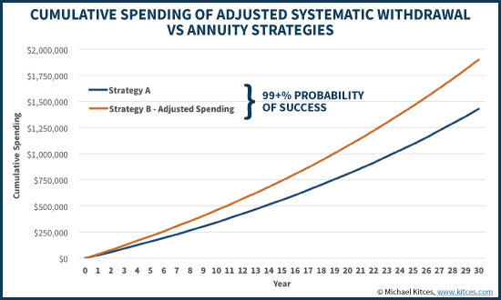
Viewed another way, the key distinction here is that while the original strategy B had a 95% probability of success and a 5% probability of failure, the magnitude of that failure wasn’t actually very severe, and it wouldn’t take much of an adjustment to stay on track (cutting from $45,000/year to $40,000/year of spending is sufficient). And even with poor returns, there is only a 5% chance the portfolio runs out of money at all, and those scenarios don’t run out until almost 28 years into retirement. Which means realistically spending would likely only need to be adjusted later – if at all – to stay on track for those final years if returns had been especially poor along the way.
Furthermore, for a 65-year-old couple, there’s a roughly 70% chance that both of them will have passed away by then anyway. Which means there’s a barely 30% probability that this 5%-failure risk is even relevant (i.e., the “joint probability” of both running out of money in their 90s and still being alive in their 90s is less than 2%). And again, if there’s still a fear that the bad returns are occurring or may occur soon, a “mere” 10% cut in spending is more than sufficient to ensure the plan stays on track, because the “failure” isn’t actually a very dramatic shortfall in the first place. Notably, even if the spending cut does have to occur, strategy B still produces more retirement spending cash flow than strategy A!
On the other hand, strategy C still turns out to be vastly inferior under the “magnitude of failure” approach, as the “bad” outcome can be very bad (flat broke by the 23rd year), and the size of the adjustment necessary to get/stay on track would be far more than “just” a 10% spending reduction.
In other words, when weighing the magnitudes of failure (and the small or large adjustments to stay on track) against the higher spending levels, strategy A turns out to be inferior to strategy B, but strategy C is worse than all of them!
Measuring Retirement Outcomes Based On Utility Functions And Risk Aversion
Notably, the conclusions of the prior section – which determined that strategy B was superior to strategy A because it provided for greater spending, and the likelihood of even needing a spending adjustment was “small”, and the magnitude of the adjustment required to get back on track was also “minor” – still presumes that the retirees are comfortable with those “small” and “minor” risks. In reality, not all retirees will be comfortable facing such trade-offs, even if the requisite spending adjustments in strategy B are likely “minor” and of remote likelihood. Or viewed another way, just because they have the financial capacity to take the risk still doesn’t mean they have the tolerance or desire to do so!
Conversely, the magnitude of potential adjustments for strategy C – which could fall seven years short on a 30-year retirement goal and possibly need 20%-30% spending cuts to get back on track – were already deemed untenable, despite the materially higher initial spending amount. Yet again, in reality at least some retirees might be willing to risk such trade-offs, and are willing to face the possibility of a “big” spending cut in order to enjoy a “big” spending increase up front.
In theory, these scenarios could be weighed against each other by trying to quantify how much “happiness” the retiree derives from greater spending, and weigh it against the “unhappiness” of having a spending cut, along with how risk-averse the retiree is to the possibility such a cut would have to occur.
And in point of fact, this is exactly what a retirement planning “utility function” is meant to measure. A concept derived from economics, the purpose of a utility function is specifically to assign a measuring unit – “utils” – to potential outcomes. More positive outcomes (e.g., higher spending levels) have higher utils. Adverse outcomes (e.g., spending cuts necessitated by the depletion or near-depletion of assets) have negative utils. On this basis, we can then compare and contrast widely-differing strategies that have a complex range of outcomes by adding up the positive and negative “utils” over time to determine which creates the most satisfying net or cumulative outcome.
Another key advantage of using a utility function is that it becomes possible to give different weights to positive versus negative outcomes – specifically, to assign greater negative weight to negative outcomes than positive weight to positive outcomes. In theory, this shouldn’t matter, because a “rational” human being should be equanimous in the face of gains or losses. In point of fact, though, the recognition that as human beings we have greater aversion to losses (more “negative utils”) than the enjoyment we gain from favorable results (relatively fewer “positive utils”) is the “Prospect Theory” first discovered by Daniel Kahneman and Amos Tversky, for which Kahneman won the Nobel Prize.
If investors were indifferent to relative gains and losses, the utility function (shown below) should be a straight diagonal line that goes from the bottom left to the top right. Instead, though, it is not. To the upper right, the line begins to flatten, revealing that we have “diminishing marginal utility” for additional wealth. In practical terms, increasing your wealth by $1,000,000 if your prior net worth was $0 is a big deal (from poverty to being a millionaire!); increasing your net worth by $1M if you already had $99M is not such a big deal (it’s not as exciting for net worth to rise from $99M to $100M). Notably, both are a $1M increase in wealth, but we weigh the latter one less favorably because its value is diminished by the prior millions already accumulated.
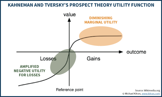
On the other hand, as the Prospect Theory graphic shows, when we lose money, we show a more “consistent” level of distress with both initial and extended losses (though the initial losses still appear to sting a little bit more).
Given that behaviorally, we do not weigh gains in the same manner as offsetting losses (and vice versa), this makes it even more important to give each its appropriate weighting in the first place.
Risk Aversion And Optimal Retirement Strategies
In the context of our three strategies, this means that the relative order of which is “best” or “worst” will depend heavily on how the retiree weighs the positive utils of having more spending and wealth, versus the negative utils of being forced to cut spending in order to avoid running out of wealth altogether.
For the highly risk-adverse retiree, who assigns an outsized negative weight (e.g., 5:1 or even 10:1) to spending cuts over spending gains, the “best” strategy is the all-annuity strategy A, which (if you believe in the security of the annuity company at least) has the smallest danger of any spending cuts, nor does it face any market volatility either (and thus no negative utils from bear markets along the way). For this retiree, anything that decreases wealth – temporarily with market volatility or permanently and necessitating spending cuts – will be inferior, and end out with a negative utility result (because of the huge weighting of any negative utils).
On the other hand, for the risk-tolerant retiree who is far more sanguine about potential losses (or simply feels more flexible to accommodate them with spending adjustments) and places a greater weighting on upside potential and enjoying more money today, strategy C could actually still be the optimal result. While as noted earlier, this strategy has a “whopping” 25% probability of failure (or at least, a 25% probability of necessitating a spending adjustment), and could require a 25%+ spending cut to get back on track, for the retiree with flexible spending who doesn’t mind the downside risk if it means a better-than-50% chance of just getting to spend more, this may be an appealing trade-off. For this retiree, strategy A once again goes from being best to worst, and strategy C is superior.
And for the retiree in the middle – who perhaps is “rather” negative about spending cuts but is willing/able to tolerate them as long as they’re “likely to be rare” and infrequent – strategy B turns out to be the “best” strategy after all, because it has the most appealing balance. For this retiree’s utility function, strategy A doesn’t bring enough upside happiness, strategy C exposes the retiree to too much downside unhappiness, and the ideal Goldilocks outcome (not too much risk, nor too little upside) is strategy B.
The ultimate point: in order to determine which strategy is “best”, given both the potential for upside wealth, and downside spending cuts, and the trade-offs entailed in pursuing greater upside at the risk of more downside, it’s necessary to “score” both the upside and the downside to objectively find the best balance between the two. And how those upside and downside outcomes are weighted will in turn depend on the retiree, and his/her preferences for managing downside risk and enjoying upside return in the first place (i.e., his/her personal utility function).
Determining The “Best” Retirement Strategy Depends On How It’s Measured
As the examples in the preceding sections have shown, determining which option is the “best” financial planning strategy can be heavily reliant on the measuring stick used to quantify the outcomes in the first place. In our choice between three strategies – annuitizing most of a portfolio for guaranteed income, taking ‘moderate’ distributions from a moderate growth portfolio, or taking large distributions from an aggressive portfolio – each strategy’s outcomes were variously best, second, or worst, depending on how the outcome was measured, as shown in the summary below.
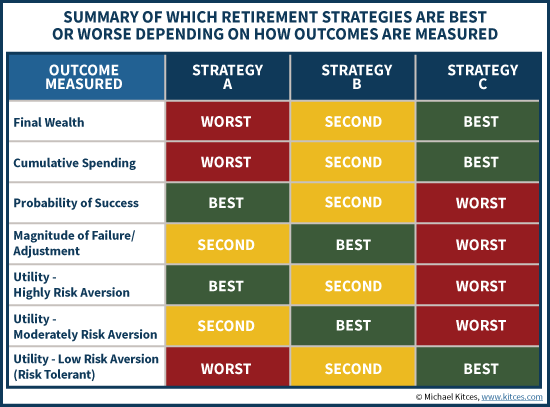
This means that careful thought about how a strategy will be evaluated is actually an essential aspect of the process in crafting financial planning recommendations. The issue is akin to what any scientist analyzing any problem has to consider: the research methodology used to analyze an issue can impact the conclusion about it, so it’s crucial to vet not just the results but the methodology itself. Otherwise, a flawed design to a research study can yield a flawed conclusion about its results.
For instance, imagine a medical study analyzing a weight-loss drug in the hopes that reducing obesity will cut down on deaths from complicating factors such as diabetes and high blood pressure. The research focuses on whether the drug leads to weight reduction, and finds that it does, concluding it’s a good drug. However, in reality, side effects of the drug itself include a significant increase in the risk of cancer and stroke! As a result, the drug does “cure” obesity but actually increases the ultimate risks of death that losing weight was meant to help minimize. In this context, if you measure “impact on weight loss” the drug is a success, but when measured by “impact on overall health” it’s actually a failure.
Of course, when it comes to financial planning, the situation is complicated by the fact most clients have multiple and complex goals and preferences. Accordingly, it’s almost impossible to establish financial planning strategies that are “objectively” dominant and superior in all situations. At best, some products or solutions might be better than others for a particular goal, or subject to particular constraints and client risk tolerance or other preferences. For instance, an emergency savings fund invested in a money market that yields 1% is clearly better than one that only yields 0.1%, and for the “core” indexing portion of a retirement account an S&P 500 index with an expense ratio of 0.1% is better than one with an expense ratio of 1%. Nevertheless, whether the high-yield money market or the low-cost index fund are “best” in the first place depends on the goals to be pursued (accumulating for retirement versus saving for an emergency fund) and tolerance for risk. With the caveat that because of our behavioral biases, even with stable risk tolerance our perceptions of these risks may be distorted in a way that inappropriate impacts our decisions (which is a discussion for another day!).
Nonetheless, the fundamental point remains that evaluating which retirement strategy is best requires a combination of both a quality process to objectively analyze the scenarios, and a careful consideration of what tools will be used to do the measuring and evaluate the outcomes in the first place, to properly fit them into a client’s preferences and tolerance for risk!
So what do you think? How do you evaluate the outcomes of potential retirement income strategies with clients? Is it based on projected wealth, cumulative spending, Monte Carlo analysis, probabilities of success, magnitudes of failure, utility functions, or something else? How do you explain these concepts to your own clients? Please share your thoughts in the comments below!


Risk tolerance is defined as “Everyone has a plan till they get punched in the mouth”. For just retired people 2015 and the gut punch of 2016 opening was an eye opener for those of us who bought and held our whole life, not knowing our bravery came from our job, did not need the money, the government would bail out the market. Then reality that 2/3 of your life is over and there might be little recover time if the market goes south. Betting on the market then seemed like a Dirty Harry question anymore.
We are out of the stock market, 50% of our money into Lifetime Income Annuity scheme which covers our basic expenses( + social security) and the other 50% we can just spend..
I read a study that the market going down hurts twice as much then if you miss it going up, they are right.
Yes there are some holes in the plan, like if one social security goes away. Some things are also a luxury, like getting an inflation rider on annuity.
We will probably get back in the market with a small amount of money to get revenge and zero out those carry over loses, but of course now its money we can afford to use.
You still have plenty of time to recover from a market downturn if you have a third of your life ahead of you. As long as you have extra money and aren’t worried about inflation you don’t need to be in stocks. One risk you do have is the financial strength of the insurance company that is getting half of your money. If they go out of business, you are out of luck. Also do not forget that one reason you are getting more than the 4% is they are paying you back your own money, your principal. If you can afford to lose the other 50% you should put some or most into the stock market. Why leave it in cash?
Another illuminating analysis Michael! I’m curious how a 50/50 immediate annuity/stock blend might have performed? It would seem that the opportunity for annuity mortality credits could offer more long-term purchasing power compared to the bond element? I would think a 40/60% annuity/stock blend might look even more attractive? And finally, how do you factor real world elderly decision-making risk or error into your analysis?
Agreed! When clients ask about annuities, I commonly hear a strategy similar to 50% of nest egg in an annuity for the “guaranteed” $30k/year income with the remaining 50% in stocks to compliment the cumulative spending/final wealth approach. That way no distributions need to be taken when markets are down while positive market returns produce “icing on the cake” spending opportunities.
We define investing success as “having money for your goals when you need it”, which typically lends to a more conservative strategy and tries to pull clients back from the allure of the “final wealth” strategy. In my mind, a client needs to demonstrate a thorough understanding of market principles before I would actually trust them to implement a high risk, strategy C-type investment portfolio and actually be able to stick with it through periods like the first half of Q1 2016. Behavior management is crucial, whatever strategy the client can actually implement without allowing their emotions to pull them off the rails is the best one to choose!
A new idea for addressing the “best interest” conunudrum is to begin a six step retirement advice process by solving for a client’s longevity risk tolerance as step one. It will require progress beyond the current industry questionnaires used for optimal asset allocations – could advisors (especially robos) have developed the scalable prudent process we now know without it? As Michael points out, the optimal asset allocation may not be in the best interest of every retiree, especially after they “take a puch” After leaving full time employment. Our pro bono think tank took a stab at it in our paper “A New Six Step Retirement Advice Process.” A major challenge was keeping it simple enough to scale to all net worth segments. We’ve posted all our ideas to our nonprofit website, which represents volunteer work done by a small group of industry veterans who would like to create a grass movement of like-minded professionals. We believe individual retirement advice should evolve to true open architecture, and we derive no revenues from the effort (an occupational hazard of objective consumer advocacy). On LinkedIn and the web: http://www.openarchitecture2020.com
I found “Can Retirement Advice Business a Profession Instead of a Sales Job” the most interesting. Everyone can measure the market/hypo risk, till your blue in the face but never met a person pushing stocks who ever lost money and was always out in the downturn, the sales job. These measurement tools are part of the Sales job.
One needs to start with the simple stuff, course no one gets a commission for this. The most ignored part in retirement planning is that cash is king and one needs to find the minimum money you have to put at risk to have a chance of meeting your goals. Course no one gets paid for cash (thats why the industry calls it trash). Realizing how much one would have to risk in the market to replace that Social Security check if you want to defer till full retirement age can be a long 4 yrs and a sobering experience (watching your 1 million drop at least 10% one time). Another realization is that the market does not care that you are only trying to make 2% when you got hit with that +10% loss on a every 3 yr regular basis. Don’t get bogged down with inflation cause read the previous sentence.
There may be some good information in there somewhere, but I got so drunk trying to read through the awful grammar, usage, and punctuation that I gave up. Sorry.
Thanks for the article, clears up a lot of questions. I guess its individual choice of where you feel most comfortable. I do have a pension option or lump sum, don’t know which to choose? Of course the fear of the pension bankrupt, even though we are insured by pbgc.
i think it’s unfortunate that a 100% stock portfolio even enters the realm of discussion of CFPs as a possible retirement income strategy. In a post MPT world, a 100% stock portfolio is arguably wrong at any age, for any person, and for any reason, let alone for the purpose of retirement income.
The 100% stock portfolio was just meant for illustrative purposes. The point is the analytical process to compare strategies, not the particular strategies illustrated here.
I could have done the same analysis comparing portfolios with 49%, 50%, and 51% in equities, and the points would all be exactly the same. The illustrations would just have lines so close together it would be hard to distinguish the magnitude of the differences is all. 🙂
– Michael
Ahh ok, and thanks for the follow-up comment. Yeah I just wouldn’t want someone to be tempted by its “pros”, then end up losing a portfolio with no human capital left to replace it with.
I’m not too worried that a retiree is going to invest their entire life savings into 100% in equities based on one example from one random blog article on the internet. If they do, I think there are probably some other issues involved. 🙂
– Michael
Yeah sure they probably won’t. But this isn’t a random blog post from just anyone. 😉
Sadly, it’s not as crazy or rare as it would seem that it should be. I’ve read many sad stories and testimonies over the years as I was plenty active in following finance in both bear markets of the last decade. Folks who were not only all equities, but even some stories of folks being near 100% tech in the 2000 crash, post retirement.
Success and Failure, Capacity and Tolerance, Pain and Gain, Utility and Aversion … all summed up nicely. Now, if this is an IRA behave like a Fiduciary and do what is in the best interest of the Client.
Where do you get the 3% on immediate annuity? Long term averages for a single 65 year old male is approximately 10%. I get that you used refund of premium but that still brings it nowhere near 3%, maybe closer to 7%. And if you plan far enough ahead using the annuity in conjuction with a life insurance policy, that would provide the highest return of them all, with the policy used as the vehicle of wealth transfer. (Also questioning the 6% from all stock portfolio, as you’re correct, that provides far and away the highest probability of failure, seems that a more comparable number to use would be 3 to 4%). The point I’m trying to make is if you want to use “today’s numbers” on the annuity side, you have to use it across the board, and using today’s numbers means a far lower distribution on the all stock, or even the balanced, portfolio.
I’m referring to the internal rate of return of the annuity, not its payout rate. A $100,000 single premium immediate annuity that gives you a $6,000/year payment is NOT a 6% return. It’s a 6% payout rate, a large portion of which is simply a return of your $100,000 principal over your life expectancy. The internal rate of return of the cash flows over life expectancy gives you a true return estimate, which is where a number like 3% comes from.
– Michael
I’m sorry, but that makes ZERO sense. In your first few paragraphs, you said “spending 30k per year from an immediate annuity”, and now you’re saying you use the IRR? Why? You changed the rules there. When someone does an immediate annuity, they don’t care what the IRR is, they care what the income they get paid is. So if they’re getting 60k, but spending 30k, where does the remainder go? Cash? Investments? A build up for another annuity down tthe line? Or thin air? It seems in your current example the answer is thin air. Maybe I’m wrong, but I’m not seeing it. I appreciate the research you’ve done, I just feel like the results are flawed.
Jason,
Sorry for the confusion here. I was responding to several comments and thought this was related to another we did about annuities that were looking at IRR.
The example here is not a 3% payout. It’s a 3.3% payout, which is $30,000/year on a $900,000 contribution (as I indicated the assumption that 90% is allocated to the annuity, with the other 10% held in cash reserves).
The example here is for an inflation-adjusted (based on CPI) annuity payout, for a 65-year-old married couple, including a cash refund guaranteed. Last I looked, this 3.3% payout is very close to the going market rate for such an inflation-adjusting lifetime annuity payout with a death benefit guarantee. (It may be off slightly as interest rates bounce around and I was trying to illustrate with reasonably round numbers.)
I hope that helps a little?
– Michael
What would the results be for a very conservative 20/80 portfolio? The temptation is to say it’s like A but I doubt that’s the case….