Excel Spreadsheet Productivity Tips For Financial Advisors

 Using Excel As A Financial Advisor

Excel is a tremendously popular spreadsheet software among financial advisors. Whether it is the primary means of conducting financial planning and/or investment management analysis, a tool for ad hoc planning, or simply used for other business management purposes, odds are almost every financial advisor will use an Excel spreadsheet from time to time.

And there are good reasons for this, as Excel is an incredibly powerful tool. However, like all tools, how effective and efficient Excel is in helping you get your work done depends on your skills and knowledge using it. The goal of this post is to serve as an introduction (or refresher) on some of the more common uses of Excel among financial advisors, including common formulas and keyboard shortcuts to use it more efficiently.

Doing Time-Value-Of-Money (TVM) Calculations

Time-Value-of-Money (TVM) calculations are one of the most fundamental building blocks of financial planning and investment management analysis. Being able to quantify the fact that a dollar today is worth more than a dollar tomorrow is useful in a wide range of applications, including helping clients compare investment alternatives, projecting the value of wealth accumulation over time, and even making important career decisions.

While most advisors learn to do TVM calculations using a physical financial calculator like the TI BII Plus, HP 10bIl+, or HP 12C, the unfortunate reality is that these tools aren’t very common or useful outside of a classroom or testing environment. In the real world, you are much more likely to be using a desktop or laptop computer with a spreadsheet or possibly working on it collaboratively with others (e.g., via Google Drive, Office 365, or Dropbox), but you may not have experience applying the same TVM formulas through Excel.

Fortunately, the mechanics are all the same and Excel is even faster and more powerful once you get the hang of it, but there can be a learning curve.

The Basic TVM Excel Functions

While it can be expressed in several forms, all advisors should be familiar with the basic TVM formula:

FV = PV * (1 + i)ⁿ

Where:

• FV = Future Value
• PV = Present Value
• r = rate of return (you may know this as “i” from HP calculators or “I/Y” from TI calculators)
• n = number of periods

In the CFP curriculum, prospective CFP certificants are typically taught that if you know three out of the four, you can solve for the fourth. (Or once payments are included, if you know four out of five, you can solve for the fifth.)

Similarly, the same opportunity exists in Excel. And not merely by brute-force projecting out the growth of an account balance over time, line by line, but simply by using an Excel function – a shortcut, that simply takes the key terms as inputs, and solves automatically for the remaining one. In fact, there is one Excel function for each of the main five components of the TVM calculation – FV, PV, i, n, and PMT (for the ongoing payments being added or subtracted) – to fully replicate what can be accomplished using a financial calculator:

• PV(rate, nper, pmt, [fv], [type])
• FV(rate, nper, pmt, [fv], [type])
• RATE(nper, pmt, pv, [fv], [type])
• NPER(rate, pmt, pv, [fv], [type])
• PMT(rate, nper, pv, [fv], [type])

For any of these formulas, start out by clicking an empty cell, typing the equals sign (which signifies the start of a formula, which may include a function), and then the capital letters associated with the function you want, and then Excel will guide you through the rest of the input. For instance, if you type “=PV” you will see the following pop-up in Excel:

This will allow you to see what functions are available that begin with those characters and what the function does. You can double click on one of the available functions with your mouse, or, if you’ve typed the function you want properly, just simply type a left parenthesis in order to use the function. Once you type “=FV(“ you will see the following:

Once you begin using the function, Excel will guide you through the process of adding each of the inputs you need to get a result. To enter the variables, simply separate each number with a comma. So, for instance, suppose I want to find the value of a $100,000 portfolio if it grows for 10 years at 8% per year. I would enter the following: “=FV(0.08,10,0,-100000,0)”

Press “Enter” (or click elsewhere) and Excel will return the proper result of $215,892.50. Notably, “type” serves the same role as the “BEG/END” option on many financial calculators (0=end; 1=beginning), but if you forget this, Excel provides a reminder as you fill in the function. And if you don’t fill in anything – as the parts of the formula in [brackets] are optional – Excel will simply assume a value of zero (which defaults to a PV of 0, and a payment type of end-of-period payments).

The other TVM functions operate in a similar manner based on what information you have and what you are trying to solve for. Like other financial calculators, do remember that PV and FV should be opposite signs of one another – for instance, in the above example, the initial $100,000 portfolio was shown as -100000 to signify the cash outflow INTO the portfolio, such that the final result coming back was a positive $215,892.50. Also, bear in mind that NPER and RATE need to be expressed based on consistent time periods. As an example of the latter, if we wanted to solve the prior example compounded monthly instead of annually, then NPER=120 (for 12 months per year times 10 years) and RATE=0.08/12. In fact, you can even type mini-formulas into the function to fill out the terms.

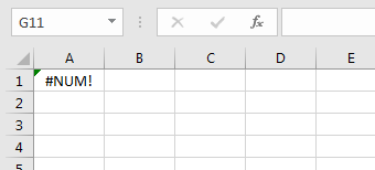
Also, when using the RATE function, one of the inputs is “Guess”. You don’t have to provide an input here (Excel will assume 10% if you don’t), but this is just to help Excel converge on a solution (as mathematically, guessing a viable rate of return for a series of cash flows requires a blind leap!). If Excel is failing to converge on a solution – it can’t actually figure out the “rate” that works, without some help (i.e., a guess that at least gets it decently close), you will get a result like this:

Of course, part of what makes Excel a powerful tool is that spreadsheets can be set up so that values can be changed, calculated, or updated automatically. There are lots of ways this can be done.

For instance, by using cell values within the function, we can easily create a simple calculator that allows us to determine future values while quickly changing inputs.

As the formula above shows, the “Future Value” cell is the calculation of FV, but now the inputs are OTHER cells (for the rate, n, and PV, as the PMT is still assumed to be zero). The significance of this approach is that now, if the advisor changes any of the numbers in the Present Value, Rate of Return, or Years cells (currently $100,000, 8%, and 10, respectively), the Future Value cell with the FV function will instantly update with the newly calculated result!

How To Do Discounted Cash Flow (DCF) Calculations – IRR and NPV

In situations where the ongoing cash flows are perfectly even, the aforementioned PV function can determine the value of a series of cash flows over time. However, when the cash flows are uneven in amount or irregular in timing, the standard TVM functions like PV no longer fit the data.

To determine the discounted present value of uneven or irregular cash flows, two particularly useful functions for financial advisors are the Net Present Value (NPV) and Internal Rate of Return (IRR). In the financial planning context, these are highly relevant in situations like comparing Social Security claiming decisions (which have differing and irregular cash flows), or trying to choose between a pension or lump sum alternative (to determine the return that the lump sum would have to earn to replicate the pension).

• NPV(rate, value1, [value2], …)
• IRR(values, [guess])

Comparing Social Security Strategies Using NPV

Suppose you are trying to evaluate the age at which a client should claim Social Security. You want to evaluate the strategies of claiming early (age 62), full retirement age (age 66), or delaying (age 70) for a single individual about to turn age 62. If the individual claims early, they receive $22,500 per year, at FRA they receive $30,000 per year, and at age 70 they receive $39,600 per year.

A simple table can be set up as follows:

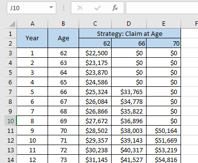
In this case, an inflation COLA (Cost-Of-Living Adjustment) of 3% was assumed. Of course, not only do we need to inflate the ongoing series of cash flow received for the individual who starts at age 62, but we must inflate the future benefits as well (e.g., benefits claimed at FRA can be calculated with “=FV(0.03,4,0,-30000,0)” to determine what that $30,000/year payment would be in 4 years at a 3% COLA).

Once we have created the table, then we can use the net present value function to determine NPV of each series of cash flows based on a specified discount rate, and based on an assumption of how long the payments will continue.

Suppose we decide to use a life span of 90 and a discount rate of 6% (based on the opportunity cost of what the funds could earn in the retiree’s conservative portfolio) in this scenario. Then, in order to calculate the NPV, we would use the function “=NPV(0.06,C3:C31)”.

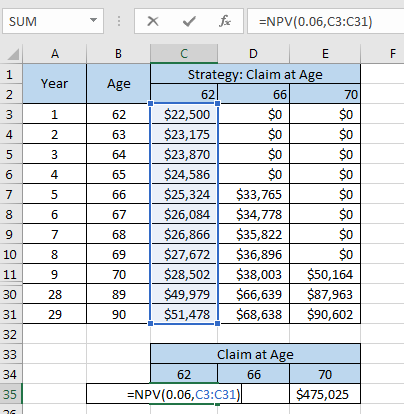
In this example, “C3:C31” represents the entire stream of cash flows (note: rows for ages 71 through 88 are included, but hidden, in the graphic above, to save space). It’s important to remember that any zero years should be included in the range selected to calculate an NPV. So, in this case, in order to determine the NPV at FRA, the formula would be “=NPV(0.06,D3:D31)”, fully capturing all four of the zero-payment years, in order to recognize that the cash flows should be appropriately discounted for how long the retiree had to wait to start getting any checks.

Another way to analyze this scenario is using IRR. For example, the decision to wait four years (from age 62 to 66) effectively means the retiree “gives up” four years of (COLA-rising) payments, in exchange for the higher payments that result beginning at age 66. Accordingly, Column E in the graphic below shows just the difference in payments between claiming at age 62 vs 66, where the cash flows are negative in the early years (when waiting results in “lost” money not received), and then turn positive once the delayed-and-now-higher payments begin. Based on this series of (differential) cash flows, we can calculate the “internal rate of return” that would be necessary to equalize them. Or viewed another way, the IRR is the hurdle rate that would need to be cleared in order to come out ahead taking benefits earlier and investing them.

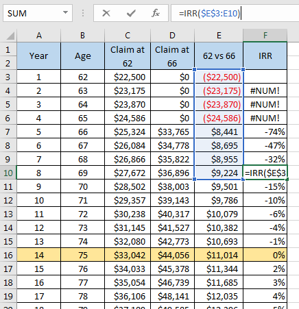
(Note: Rows from ages 70 through 85 are included in the spreadsheet, but hidden in the graphic above.)

Of course, this is only the IRR of delaying Social Security if the retiree lives all the way to age 90. Another way to analyze the situation, using IRR, is to calculate the IRR from the start (age 62) through each possible year. Which reveals how the IRR of delaying Social Security gets better and better the longer the retiree lives; what is initially a negative IRR eventually breaks even (reaches 0%) after 14 years, and then turns increasingly positive from there.

In this case, the IRR function is used with the range selected as all cash flows. As you can see in the graphic above, cell F10 contains the function: “=IRR($E$3:E10)”. Do note that the dollar signs before “E” and “3” serve as anchors fixing both the row and column (press F4 while inputting the relevant part of the formula to quickly anchor a cell). By doing so, the formula can be copied all the way down the column, from Cell F7 to Cell F19, and the formula automatically updates, recognizing that as the formula is copied into each new row, it should extend to capture that new row, but will always start at E3 (the first year of the analysis, anchored as $E$3). Thus, it’s only necessary to type the formula once, and then copy-and-paste it for all the rows.

Also, notice that we get a result of “#NUM” prior to age 66. The reason for this is because we have no positive cash flow yet, which means there is no possible IRR that can turn only a series of negative cash outflows into a positive result! Notably, the results from age 66 to 67 also originally returned “#NUM”, but this was because Excel wasn’t able to converge on a solution without providing a guess. Guesses of -0.5 and -0.7, respectively, were given in order to get Excel to converge on solutions (which were -0.74 and -0.47, or -74% and -47%).

What the results above are telling us is that is that at age 75 the breakeven point in terms of nominal dollars (0% IRR) is reached. Had the individual in this scenario died at age 73, they would have needed to earn an annualized -4% return in order to breakeven taking their benefits early and investing them. However, at age 78 that same individual would have needed to earn annualized returns of 4% in order breakeven compared to the higher annual benefits received by delaying.

Pension Vs Lump Sum Analysis Using NPV And IRR

Discounted cash flow analyses are also useful for analyzing various pension-vs-lump-sum options. After all, when an individual has a choice between the two, choosing the pension is the functional equivalent of “paying” the lump sum, in exchange for a lifetime stream of (pension) payments. Which allows for an IRR analysis, similar to the one used for Social Security above.

For instance, assuming an individual has the choice between a $300,000 lump sum or a lifetime annuity of $20,000, we could set up an Excel spreadsheet table as follows (ultimately extending out to the maximum age of the desired analysis):

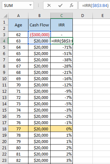
Again, the same IRR function and anchoring is used, with the function in cell C4 being “=IRR($B$3:B4)”. No guess was needed in order to get Excel to converge on a solution this time.

What the results are telling us here is that age 77 is the breakeven point in nominal dollar terms (which we can verify given that 15*$20,000=$300,000). However, by age 82, and individual would have needed to earn an annualized return of at least 3% on that $300,000 in order to come out ahead taking the lump sum and investing the proceeds (instead of just getting the $20,000/year). The longer the pensioner lives, the higher the IRR, and the harder it is to achieve a comparable rate of return (at least, not without taking on an undesirable level of risk). Which helps to illustrate that the relative value of a pension vs a lump sum is highly contingent on both how long the individual lives, and what rate of return could have been earned (i.e., the opportunity cost of the lump sum had it been available to invest).

Of course, these are simplistic comparisons, and there’s much more we can do to maximize pension versus lump sum decisions, but the purpose here is simply to provide the basic overview of how you would set up the comparison using an Excel spreadsheet.

Keyboard Shortcuts For Using And Getting Around Excel

When financial advisors use an Excel spreadsheet intensively, the sheer amount of typing into cells, and clicking around with the mouse to navigate, can become time-consuming. Fortunately, though, the reality is that Excel has extensive keyboard shortcuts.

Most everyone is familiar with simple keyboard shortcuts such as Ctrl + C to copy, and Ctrl + V to paste, but if you are a heavy user of Excel and aren’t familiar with the many additional shortcuts available, do yourself a favor and get rid of your mouse for a month and force yourself to navigate Excel with the keyboard. Seriously. Unplug your mouse and use nothing but the keyboard. You won’t regret it.

While there are far more possible keyboard shortcuts than can be covered here – many of which depend on how you use Excel – here are a few particularly useful shortcuts you may want to consider learning as a financial advisor:

• Ctrl + [Arrow Key]
  • Holding control and pressing an arrow key (e.g., the Right arrow, or the Down arrow) will jump to the nearest filled cell or across continually filled cells in that direction. This can be particularly useful when navigating spreadsheets with hundreds (or more!) rows of data. If you are near the top row of the data and want to quickly get to the bottom of the data in that column, just push Ctrl + Down (Arrow) to instantly jump to the bottom. Practicing this is one of the keys to getting good at moving around spreadsheets without a mouse.
• Shift + [Arrow Key]
  • Holding shift while navigating with the arrow keys will allow you to select (highlight) an area while anchoring the selection in the cell you were originally in when you pushed shift.
• Ctrl + Shift + [Arrow Key]
  • Many shortcuts are most useful when combined with one another or used in some type of sequence. This is one example of combining the two shortcuts above. Quickly select an entire column of continuous data by pressing Ctrl + Shift + Down (assuming you are starting at the top). Again, this is often much faster than trying to select cells with your mouse, and dragging down to the bottom of the column (especially if you have a lot of data!). You can also use this in multiple directions at once [e.g., Ctrl + Shift + Down + Right (select continuous block of cells both down and to the right) …or… Ctrl + Shift + Down – Ctrl (i.e., release Ctrl but keep holding shift) + Right (select two columns of continuously filled cells)].
• Shift + Space
  • Highlight an entire row. This is particularly useful if you want to quickly modify or delete an entire row.
• Ctrl + Space
  • Similar to highlighting an entire row, this shortcut allows you to highlight an entire column.
• Alt + E + D (Holding Alt, and pressing E and then D sequentially)
  • This shortcut deletes the cells in a selection (i.e., actually removes the cells and gives you the option of how to shift the ones that are left…if you just want to delete the contents inside a cell, just hit “Delete”). This can be particularly useful when combined with Shift + Space or Ctrl + Space to quickly delete an entire row or column.
• Alt + I + R (Holding Alt, and pressing I and then R sequentially)
  • Insert a row. Nice shortcut for when you want to quickly add cells to a spreadsheet.
• Alt + I + C (Holding Alt, and pressing I and then C sequentially)
  • Insert a column. Same as above, but adds a column instead.
• Ctrl + C → Alt + E + S
  • This is a combination of two shortcuts. Ctrl + C (copy) then Alt + E + S which opens special paste commands. From this prompt, you can manually select things such as to paste only values, formats column widths, etc. However, the underlying special pastes also have shortcuts, which can allow you to paste how you want even faster.
• Alt + E + S + V
  • Paste values.
• Alt + E + S + T
  • Paste formats.
• Alt + E + S + W
  • Paste column widths.
• Alt + E + S + F
  • Paste formulas.
• Alt + E + S + E
  • Paste transpose (i.e., convert a row into a column nor a column into a row). For instance, if a client gave you a spreadsheet that included annual income across columns but you wanted to insert annual income into an existing spreadsheet as rows, you could simply transpose the data rather than rewriting it (which can save a lot of time if you have a lot of data!).
• Ctrl + Shift + Down + Right → Ctrl + C → (navigate) → Alt + E + S + T → Alt + E + S + W
  • Suppose you have two identical sized tables, but you want to format Table 2 exactly the same as Table 1. Format painter is one quick way to do this. But an even faster way (once you get good at it) is the combination above. Perhaps the particular sequence is practical for how you use Excel, but it’s a good example of how shortcuts can be combined and used sequentially in order to get the biggest efficiency gains.
• Ctrl + 1
  • Access number formats.
• Ctrl + Shift + 1
  • Format the highlighted cell(s) as number
• Ctrl + Shift + $ (the number 4 is the $ when holding shift)
  • Format the highlighted cell(s) as dollars. (Handy to quickly format financial projections with dollar signs!)
• Ctrl + Shift + % (the number 5 is the % when holding shift)
  • Format the highlighted cell(s) as a percentage.
• Alt + =
  • Auto-sum row or column.
• Ctrl + H
  • Find and replace.
• Ctrl + ~
  • Show all formulas in every cell (instead of just showing the numbers/results).

Ultimately, how you personally use Excel as a financial advisor, and the kinds of problems you solve or analyses you conduct, will dictate what opportunities there are to use Excel more effectively or efficiently. However, if you spend any significant amount of time using Excel, there’s probably a shortcut or two that can save you a lot of time. And, of course, we’ve only scratched the surface here. Excel has all sorts of features—vlookup, solver, VBA, form controls, etc.—that can make Excel an even more powerful tool for a financial advisor.

If you are looking for a handy cheat sheet of Excel shortcuts, Breaking Into Wall Street has put together a nice summary. And, unfortunately, if you happen to use a Mac there are some different shortcuts to learn, but Wall Street Prep also has a good summary of both Windows and Mac Excel shortcuts.

So what do you think? Do you have any tips for using Excel as a financial advisor? Have you taken some time to make sure you really know how to be efficient with the software? Please share your thoughts in the comments below!