Does Monte Carlo Analysis Actually Overstate Tail Risk In Retirement Projections?

Monte Carlo Analysis And Relying On A Normal Distribution

While already included in most financial planning software solutions, Monte Carlo analysis remains a somewhat controversial projection tool for financial planners, due to the fact that it commonly relies on a normal distribution to project the probability of future returns in a world where many have suggested that returns are not actually normally distributed. Which raises the question of whether or to what extent Monte Carlo analysis projections might be understating the risk of a retirement plan?

To evaluate this question, it helps to first revisit what the normal distribution is, and how it actually works.

The normal (or Gaussian) distribution is one of the most commonly used distributions in both natural and social sciences. From a statistical perspective, there are many neat and useful characteristics of a normal distribution, including the fact that distributions of many naturally occurring phenomena—such as human height, IQ scores, and measurement errors—can be approximated with a normal distribution.

One of the most common ways advisors use normal distributions is in Monte Carlo simulations. A Monte Carlo simulation models future outcomes by randomly selecting returns, based on the likelihood that they occur – where the “likelihood” is quantified by the average and standard deviation of a normal distribution, which recognizes that extreme returns (to the upside or downside) are less common.

For instance, if an advisor wants to conduct a simulation assuming a 5% average return and 10% standard deviation, the following normal distribution would be produced:

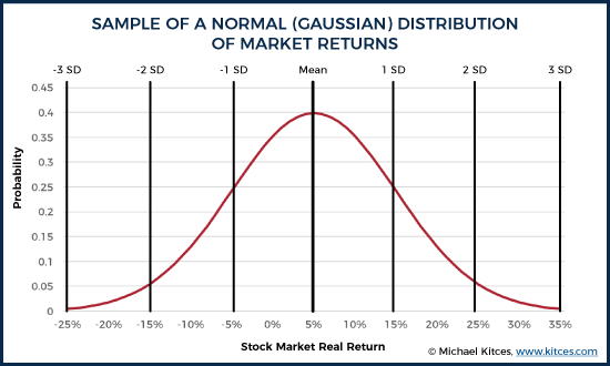
As you can see in the graphic above, the most common return that would be selected randomly is 5%, while more extreme values would come up less frequently. Specifically, in a normal distribution, 68% of the values occur within 1 standard deviation of the mean (in this case, a return between -5% and +15%), 95% of the results are within 2 standard deviations (e.g., -15% to 25%), and 99.7% of the values fall within 3 standard deviations (which would be returns from -25% to 35%). In other words, given the parameters above, returns greater than 35% or less than -25% (i.e., more extreme than 3 standard deviations), would only be expected to occur about 0.3% of the time.

However, as noted earlier, a leading criticism of Monte Carlo analyses is that “extreme” returns can occur more often than the 0.3% frequency implied by a normal distribution – in other words, the “tails” of the distribution are “fatter” (i.e., more frequent) than what a normal distribution would project, particularly to the downside (i.e., a catastrophic bear market). Although, notably, the extent to which market returns have “fat tails” depends on the time horizon involved. While many studies have shown that daily and monthly stock returns appear to have fatter tails, when projected annually (as is common in financial planning projections), the downside fat tails largely disappear.

This lack of “fat tails” in long-term annual stock returns also holds true for 60/40 portfolio returns, based on the large-cap U.S. stocks and Treasury Bills. Using Robert Shiller’s data going back to 1871, we can use a Shapiro-Wilk test to examine whether annual returns exhibit a statistically significant deviation from a normal distribution – and the findings suggest they do not. In other words, while there may be “fat tails” in the short-term (daily or monthly) return data, it averages out by the end of the year.

Comparing Historical Returns And Monte Carlo Projections

Notwithstanding the lack of fat tails evident in the data for annual-return retirement projections, many financial planners eschew Monte Carlo analysis and prefer to simulate prospective retirement plans using actual historical return sequences, which, by definition, capture actual real-world volatility (potential fat tails and all) that has occurred in the past. In fact, the entire origin of Bengen’s “4% rule” safe withdrawal rate was simply to model retirement spending through rolling historical time periods, identify the worst historical scenario that has ever occurred, and use that as a baseline for setting a “safe” initial spending rate in retirement.

We can get a sense of whether or to what extent Monte Carlo analysis understates long-term tail risk relative to actual historical returns by actually comparing them in side-by-side retirement projections.

Data available from Robert Shiller, going back to 1871, provides a sequence of actual historical returns (for large-cap U.S. stocks, and Treasury Bills) that we can use to evaluate the impact of “real-world” market volatility on retirement, and then compare it to what a Monte Carlo analysis projection would show using the same average return and volatility as that historical data.

If we assume a 60/40 portfolio of stocks and fixed income (annually rebalanced), and a portfolio that begins at $1,000,000 (to make the numbers round and easy), the starting point is to look back into the initial withdrawal rate that would have “worked” for any particular rolling 30-year period (based on actual historical return sequences). Accordingly, we find that in the worst-case scenario the “safe” spending rate was $40,766 at the beginning of the first year (with spending adjusted each subsequent year for inflation). This equates to a 4.08% initial withdrawal rate (relative to the starting account balance), reaffirming Bengen’s 4% rule.

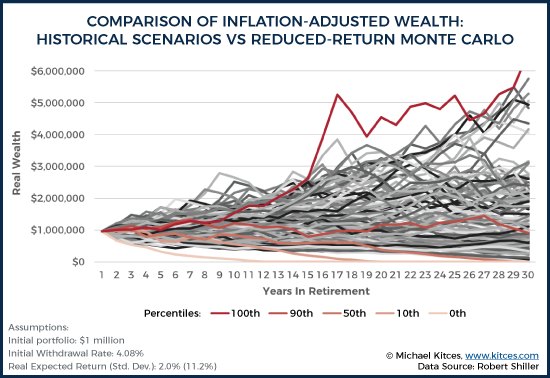
Notably, though, most of the time a 4.08% initial withdrawal rate is unnecessary. If we assume that the retiree always takes that $40,766 of initial spending and adjusts each subsequent year for inflation, we end up with the following range of wealth outcomes.

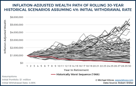
In the chart above, the worst 30-year sequence in history (beginning in 1966) is indicated in red. For that one worst-case scenario, the retiree still makes it to the end (but just barely), thus necessitating that 4.08% initial withdrawal rate. In all the other scenarios, though, the 4.08% safe withdrawal rate is actually “too” conservative, and the portfolio finishes with sometimes very substantial (inflation-adjusted) wealth left over at the end.

In fact, the retiree actually dies with more inflation-adjusted wealth than they had entering retirement in over 50% of scenarios by using that 4% initial withdrawal rate! And in 30% of scenarios, retirees would have died with nearly 200% of their initial inflation-adjusted wealth or more! In nominal terms, this means a retiree who entered retirement with $1,000,000 would have died with $4,000,000 (or more) 30% of the time, even after taking an inflation-adjusted annual distribution each year (assuming an average inflation rate of 2.5%).

Given these results based on the actual historical record, we can then re-evaluate the same retirement time period, using the same historical return data, by running a Monte Carlo analysis that uses the average return and standard deviation of the annual returns that underlie this historical time period. In this case, the data from 1871 to 2015 show that the annually rebalanced 60/40 portfolio had an average annual real return of 5.9%, with a standard deviation of 11.2%.

Using these real return and standard deviation inputs, the chart below shows various percentiles outcomes of a Monte Carlo analysis with 10,000 iterations. To see how “bad” the worst Monte Carlo scenarios are at a 4.08% initial withdrawal rate, these percentile outcomes are compared to the actual historical return sequences (which includes the historical worst-case scenario in 1966, which necessitated the 4.08% initial withdrawal rate in the first place).

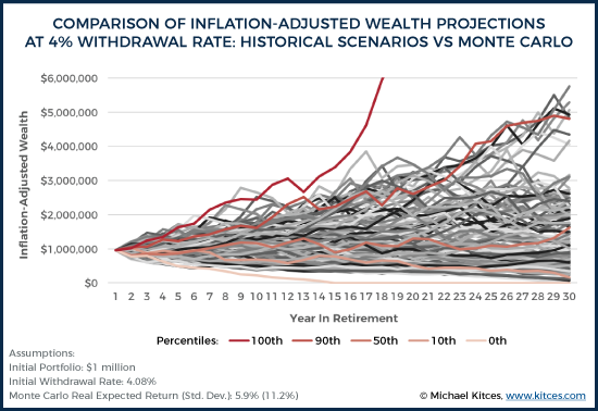
As the chart reveals, the best and worst Monte Carlo scenarios (0^th and 100^th percentiles) were actually far more extreme than any actual historical best or worst scenario. With the Monte Carlo analysis, the worst-case retiree scenario ran out of money as early as only 15 years into retirement, even though the same spending rate never actually ran out in any of the 114 rolling 30-year historical scenarios. Conversely, under the best Monte Carlo scenario, the retiree died with nearly $27 million in real wealth, even though the best case historical scenario finished with “just” $6 million of inflation-adjusted wealth at the end. The following chart summarizes the ending real wealth values at various percentiles.

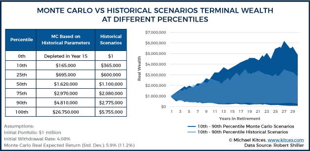
The key point is that, despite the common criticism that Monte Carlo understates volatility relative to using rolling historical scenarios, the reality, at least relative to historical scenarios, is actually the opposite – the Monte Carlo projections show more long-term volatility, resulting in faster and more catastrophic failures (to the downside), and more excess wealth in good scenarios (to the upside). In fact, the 0^th percentile historical scenario (worst case scenario, running out of money at the end of 30 years) was actually the 6.5th percentile in Monte Carlo, while the 50^th percentile historically (finishing with $1.1M remaining) was the 37th percentile in the Monte Carlo projection, and the 100^th percentile (best case scenario) historically was “just” the 93.7th percentile result with the Monte Carlo projection.

Of course, it shouldn’t be surprising that Monte Carlo comes up with more extreme best and worst-case scenarios, given that it’s based on 10,000 trials (while the historical data has only 114 series of overlapping data points), and a higher volume of random trials should yield results that are more extreme.

Nonetheless, the point remains: plans that succeed in 100% of historical scenarios may only be projected to succeed 95% of the time in Monte Carlo, suggesting that the problem may not be that Monte Carlo is understating risk, but that it is being overstated given the frequency that Monte Carlo projects scenarios that are more extreme than those that have been experienced in the past! (As it wasn’t just a 1-in-10,000 Monte Carlo scenario that was more extreme than the historical record… instead, it was 650-in-10,000!)

The Gap Between Monte Carlo And Reality: Long Sequences Without Mean Reversion

To understand why there is such a gap between the Monte Carlo results and the actual historical scenarios, we can delve further by looking at the actual sequence of real returns that underlies each.

First, let’s examine the initial 15 years of real returns of a 60/40 portfolio starting in 1966 (the worst retirement starting year of the last century):

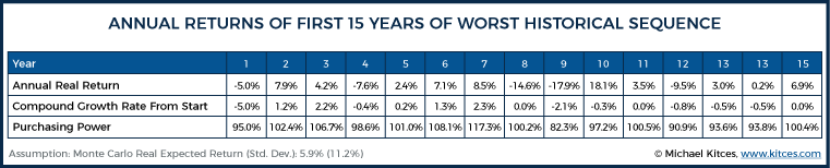
As the chart reveals, this worst-case historical 30-year sequence didn’t get off to a great start (as you’d expect, given the impact of sequence of returns). After 10 years, the average annual compound growth rate of the portfolio was negative. Which means, after accounting for inflation (and without even considering taxes or fees), a retiree with a 60/40 portfolio had already gone backward in inflation-adjusted terms. And this is before considering the impact of distributions themselves (i.e., these are time-weighted returns, not dollar-weighted). At the end of the entire 15 years, returns had still gone nowhere in real terms, and the portfolio was merely treading (inflation-adjusted) water.

By contrast, though, the sequence starting in 1966 was a walk in the park compared to the worst Monte Carlo scenario:

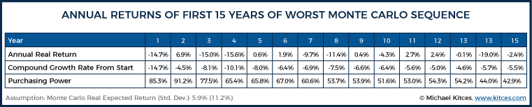
0% real returns start to sound good after looking at how extreme the worst-case Monte Carlo results were! 10 years in, the retiree has experienced a -6.6% compounded real return, which, in annualized form, somewhat masks how bad these returns truly are. In real dollars, this retiree’s portfolio would have lost roughly 50% of its purchasing power in the first decade, and by year 15, it would only buy roughly 43% of its original value! And that’s before the impact of the withdrawals themselves!

Notably, the extremes within the year-to-year annual real returns of the two scenarios are roughly comparable. The historical sequence included 14.6% and 17.9% declines, while the Monte Carlo scenario included 19.0% and 15.6% declines. What differs, though, is the sequencing and frequency of negative returns – specifically, the way in which the Monte Carlo scenario continues to string together multiple bear markets without ever having a recovery.

In the historical scenario, the 2-year decline in years 8 and 9 (which represents the 1973-74 bear market) was followed by an 18.1% rebound. In the Monte Carlo scenario, though, the portfolio started out with a substantial market decline of 14.7%, had “just” a 6.9% rebound, then experienced a 1973-74 style decline in years 3 and 4… after which there was a less-than-3% rebound, followed by another 2-year bear market. And then, after mostly flat returns for 5 years, there was another bear market. And thus, by the end, the Monte Carlo scenario eroded a whopping 57% of its real purchasing power, even though the worst actual historical scenario merely broke even on purchasing power after 15 years (which admittedly is still a horrible sequence compared to a long-term real return that averages closer to 5%/year!).

And notably, this phenomenon isn’t unique to just the worst-case Monte Carlo scenario. If we look at the worst 250 Monte Carlo scenarios (i.e., the worst 2.5% of the 10,000 trials), all of them end up with an ongoing series of extreme negative returns with little-or-no rebounds, such that they all deplete in 15-24 years. Yet again, the actual worst-case historical scenario with this spending rate still lasted for 30 years.

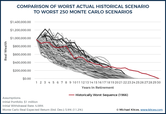
It’s not until we move up to the worst 650 to 900 Monte Carlo scenarios (i.e., the 6.5^th to 9^th percentiles) that we even find Monte Carlo results “as bad” as the actual historical record. Or, viewed another way, a 93.5% probability of success in Monte Carlo was the equivalent of a 100% success rate in the historical record!

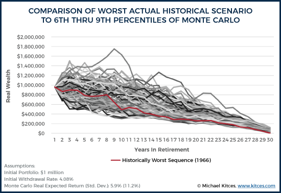
Still, even in these Monte Carlo trials, the fact that Monte Carlo analysis does not consider the natural rebound effects of markets remains evident. For instance, consider the standout iteration above that jets off by itself to the upside, approaching $1.8 million in year 8 above. In this case, the scenario started off with astonishingly strong returns for a 60/40 portfolio, as real returns were 21%, 20%, 9%, 2%, 4%, 9%, 10%, 13% over the first 8 years, which is an average annual compound real return of 10.8% for 8 years! Yet this scenario still finishes in the bottom 10% overall, because the next series of returns were equally improbable in the other direction, with the sequence of -5%, -11%, -27%, -25%, -17%, 18%, -15%, -4%, -14%, over the next 9 years, which equates to a -11.9% compounded real return for 9 years… or a 68% real decline in 9 years, far worse than even the worst actual 9-year sequence in history!

In other words, the gap that is emerging between Monte Carlo and historical market returns may not just be due to the fact that 10,000 Monte Carlo scenarios produce the potential for more extreme market declines than just 114 actual 30-year rolling historical scenarios. Instead, another distinction may be that with actual market returns, markets tend to at least pull back after several years of strong returns and to rebound after a crash. Yet, in the most extreme Monte Carlo projections, they often just keep rising or declining in dramatic fashion, regardless of how expensive or cheap the stocks are getting.

Tail Risk, Momentum, and Mean Reversion In Stock Market Returns

Mathematically, Monte Carlo analysis assumes that each year’s returns are entirely independent of the prior year(s). In other words, whether the prior year was flat, saw a slight increase, or a raging bull market, Monte Carlo analysis assumes that the odds of a bear market decline the following year are exactly the same. And the odds of a subsequent decline in the following years also remains exactly the same, regardless of whether it would be the first or eighth consecutive year of a decline!

Yet, a look at real-world market data reveals that this isn’t really the case. Instead, market returns seem to exhibit at least two different trends. In the short-run, returns seem to exhibit “positive serial correlation” (i.e., momentum – whereby short-term positive returns are more likely to be followed by positive returns, and vice-versa), and, in the long-run, returns seem to exhibit “negative serial correlation” (i.e., mean reversion – whereby longer-term periods of low performance are followed by periods of higher performance, and vice-versa).

Because Monte Carlo projections are long-term projections spanning multiple years (or decades), it is the “negative serial correlation” (i.e., mean reversion) which may cause the “tails” of Monte Carlo projections to actually be more volatile and extreme than anything in the historical record. In other words, because most Monte Carlo analyses don’t account for mean reversion, this specific aspect of Monte Carlo projections will actually tend to overstate tail risk (not understate it!).

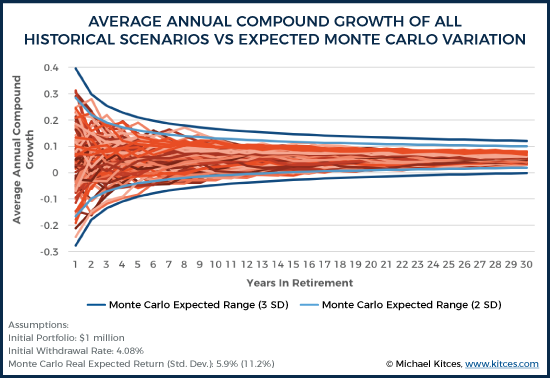
For instance, the chart below shows the average annual compound growth rates (in real returns) of all scenarios in the historical record, and compares these to what Monte Carlo analysis would predict at the 2 standard deviation and 3 standard deviation levels of compound returns, simply using an (annually independent) normal distribution based on the historical mean and standard deviation. If fat tails were present in the returns of a 60/40 portfolio, the most extreme historical records should fall outside of the 2 standard deviation Monte Carlo bands about 5 percent of the time; yet, as the results appear to reveal, over 30-year time periods, historical markets have never fallen outside the 2 standard deviation thresholds, indicating long-term returns may actually exhibit less volatility than Monte Carlo analysis would predict! Which, in turn, means that Monte Carlo analysis may actually overstate the tail risk in long-term returns!

Do Monte Carlo Retirement Projections Overstate Or Understate Tail Risk?

In the case of highly leveraged hedge funds, the reality is that it doesn’t matter if returns are mean-reverting in the long run, because a margin call can end a highly leveraged investor in a single day or week (as occurred in the famous case of Long-Term Capital Management). However, financial planning projections typically do rely on annual data (with annual withdrawals), not daily (or weekly or monthly) data. And, in the annual context, these kinds of extreme events are actually just a short-term distraction that vanish in long-term data! Instead, the problem is actually that Monte Carlo analysis may be overstating the dangers of failure by overestimating the frequency of long-term tail risk (in addition to overstating the potential upside in good scenarios)!

And this distinction is especially important given the popular tendency of financial advisors to reduce long-term return assumptions as a way of adjusting for Monte Carlo’s perceived understatement of tail risk. Recent academic research, such as the 2017 article Planning for a More Expensive Retirement by David Blanchett, Michael Finke, and Wade Pfau, urges that it is important to consider the planning consequences of forward-looking real portfolio returns in the 0% to 2% range (compared to a historical average of 5.9% for a 60/40 portfolio).

To explore the potential impact of these reduced return assumptions, we can evaluate 10,000 new Monte Carlo simulations using the same standard deviation (11.2%) but a lower mean real return (2%), and then compare the Monte Carlo results to actual historical scenarios.

As the results show, when long-term real returns are reduced to just 2%, then 50 percent of all Monte Carlo trials end up being worse than anything that has ever actually happened in history. In other words, assuming 2% real returns in Monte Carlo analysis may imply there is a 50% probability of a long-term path worse than the Great Depression or the stagflationary 1970s! The full comparison at various percentiles is included below.

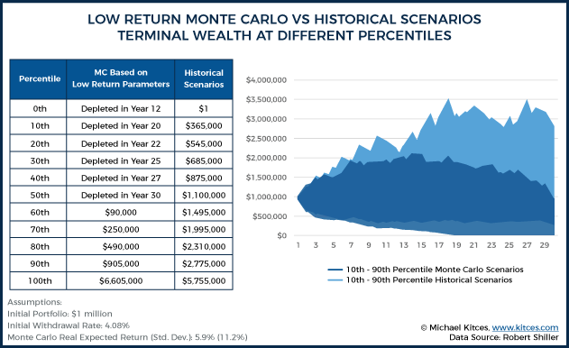
And for those who assume the low end of Blanchett, Finke, and Pfau’s spectrum – with real returns at 0% – then Monte Carlo analysis would show that 82% of Monte Carlo trials are worse than anything that has ever happened in US history!

Notably, this doesn’t mean that the alternative of ignoring today’s low yields and high valuation is better. But it is important to understand the full impact of reduced return assumptions in a Monte Carlo analysis, particularly recognizing that Monte Carlo analysis already projects more long-term tail risk by not accounting for mean reversion. And, thanks to mean-reversion, it may be the case that even reduced 10-year returns don’t necessarily imply dramatic reductions to 30-year returns, though the sequence remains important. Ideally, Monte Carlo analysis tools would allow a combination – such as reduced real returns for 10 years, followed by normalized returns with mean reversion – but, unfortunately, no financial planning software is yet built to provide such regime-based Monte Carlo projections.

The bottom line, though, is simply to recognize that despite the common criticism that Monte Carlo analysis and normal distributions understate “fat tails”, when it comes to long-term retirement projections, typical Monte Carlo assumptions actually overstate extreme outcomes relative to historical returns due to the failure to account for mean reversion – yielding a material number of projections that are worse (or better) than any sequence that has actually occurred in history. Or, viewed another way, Monte Carlo analysis may actually project worse returns than those underlying the 4% safe withdrawal rate research, and choosing a Monte Carlo analysis with a 95% probability of success may unnecessarily constrain a retiree's spending by failing to account for the reality that bear markets do eventually fall enough that stocks get cheaper and begin to recover!

Which means, perhaps it’s time for financial planning software to do a better job of either allowing advisors to do retirement projections showing actual historical return sequences, or better show what the range of returns really are within a Monte Carlo analysis, in order to help prospective retirees understand just what a 95% Monte Carlo “probability of success” really means!

So what do you think? Do you still believe Monte Carlo analyses understate tail risk… or overstate it? Is it possible that utilizing low return assumptions just overstates tail risk further? How do you set Monte Carlo parameters for your clients? Please share your thoughts in the comments below!