How Different Monte Carlo Models Perform In The Real World: Assessing Quality Of Predictiveness In Retirement Income Forecasting Models

When developing advice, financial advisors often depend on probabilistic forecasts that are usually based on Monte Carlo simulations. But we often forget to ask the obvious question: Are those forecasts any good?

When advisors say that a plan has, for example, “an 80% probability of success”, they naturally assume their forecasting model aligns well with the real world and provides a reasonable basis for making good decisions. They assume that a plan that they estimate will fail 20% of the time won’t, in fact, fail 40%, 60%, or 80% of the time in the real world (gross underestimates of risk). They assume that a plan with a dire 30% probability of success won’t actually succeed 60% or 80% of the time (gross overestimates of risk).

But research assessing how well probabilistic forecasts in financial planning perform in the real world is limited. This is an important issue: If we’re going to give advice on consequential life decisions and base that advice at least in part on probabilistic forecasts, we should pay close attention to how those forecasts perform in the real world, use the approaches that perform the best in practice, and look for ways to improve them.

We recently conducted a study that addresses this issue and found that the most commonly used approach to forecasting in financial planning – traditional Monte Carlo simulation – is prone to troubling errors and may not perform as well as other available alternatives. However, we’ll also see that no method comes anywhere close to perfection, which necessitates an ongoing process of monitoring, updating, and adjusting plans.

What Makes For Good Probabilistic Predictions?

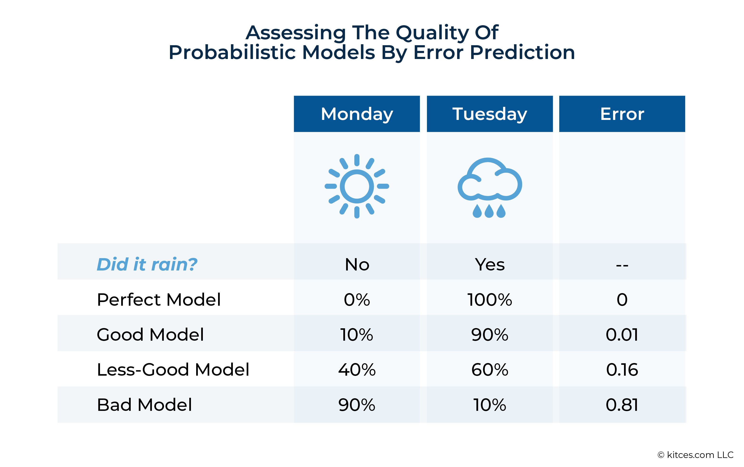
Because so many things are uncertain but not entirely unpredictable, probabilistic predictions are common in today’s world. A perfect model for forecasting rain would predict a 100% chance of rain on days when it rains and a 0% chance of rain when it doesn’t. But the world is too complex for this kind of perfection, so instead, weather models assign probabilities between 0% and 100%: There’s a 10% chance of rain on Monday, 90% on Tuesday, etc.

Models that make probabilistic forecasts can’t be ‘perfect’, but they can be better or worse than alternative models. If it tends to rain on days when a model predicts a 90% chance of rain, and it tends not to rain when the model puts that probability at 10%, that’s a pretty good model. It’s better than a model that predicts the chance of rain at 40% and 60%, respectively, in these same situations and much better than a model that predicts a high chance of rain on dry days and a low chance on wet ones.

By looking at lots of actual probabilistic forecasts and the corresponding real-world outcomes, we can measure the error of the model’s predictions. By comparing error across different models (where low error is better), we can see which model best helps us decide, say, whether to bring an umbrella to work.

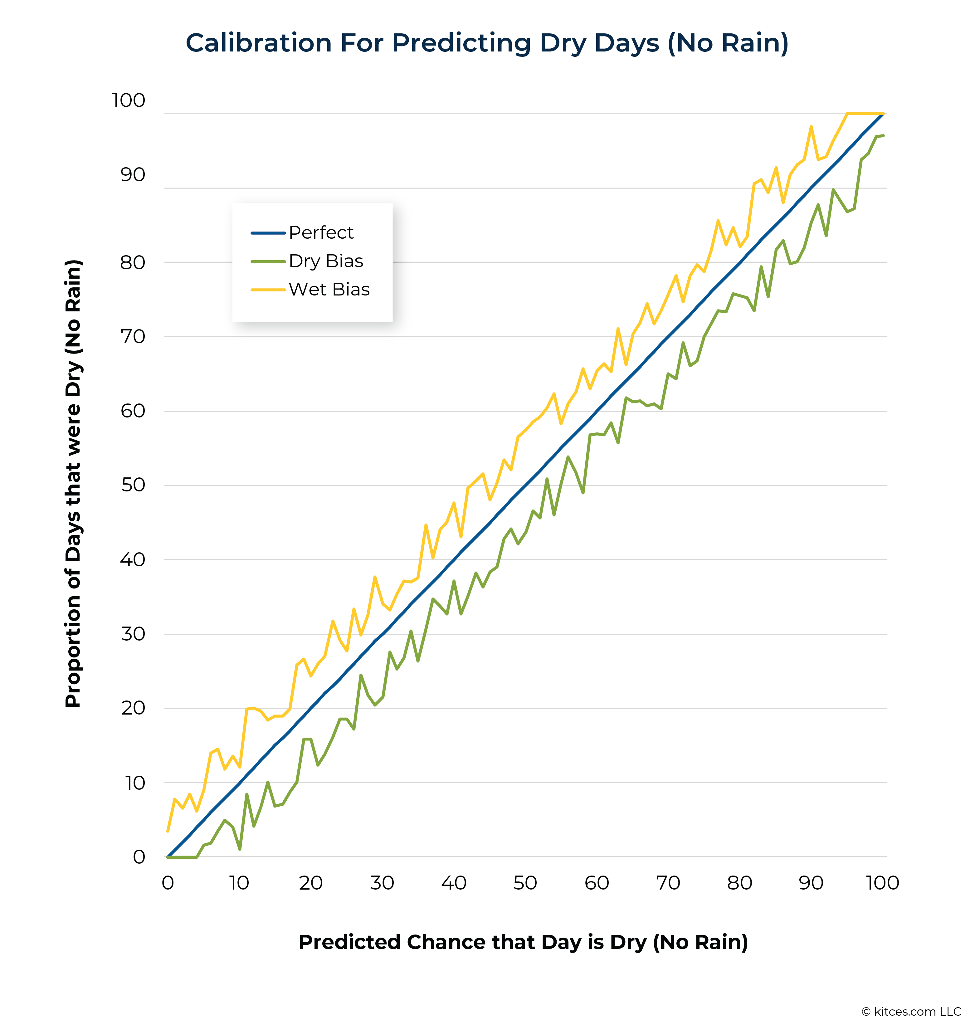
The error measurement above is very useful, but there is another way to figure out if a model is any good and where it has flaws. Suppose we have 100 instances where a model forecasted a 90% chance of rain. If it rained on 90 of those days, we have a good model (at least for days when rain is likely). In statistical jargon, we would say that this model is ‘well-calibrated’ for high-rain periods.

While good calibration for particular types of situations (e.g., rainy days) is good, a model that is well-calibrated across a range of situations is even better. For example, we’d want it to rain about 10% of the time when we predict a 10% chance of rain, about 60% of the time when we predict a 60% probability of rain, and so on.

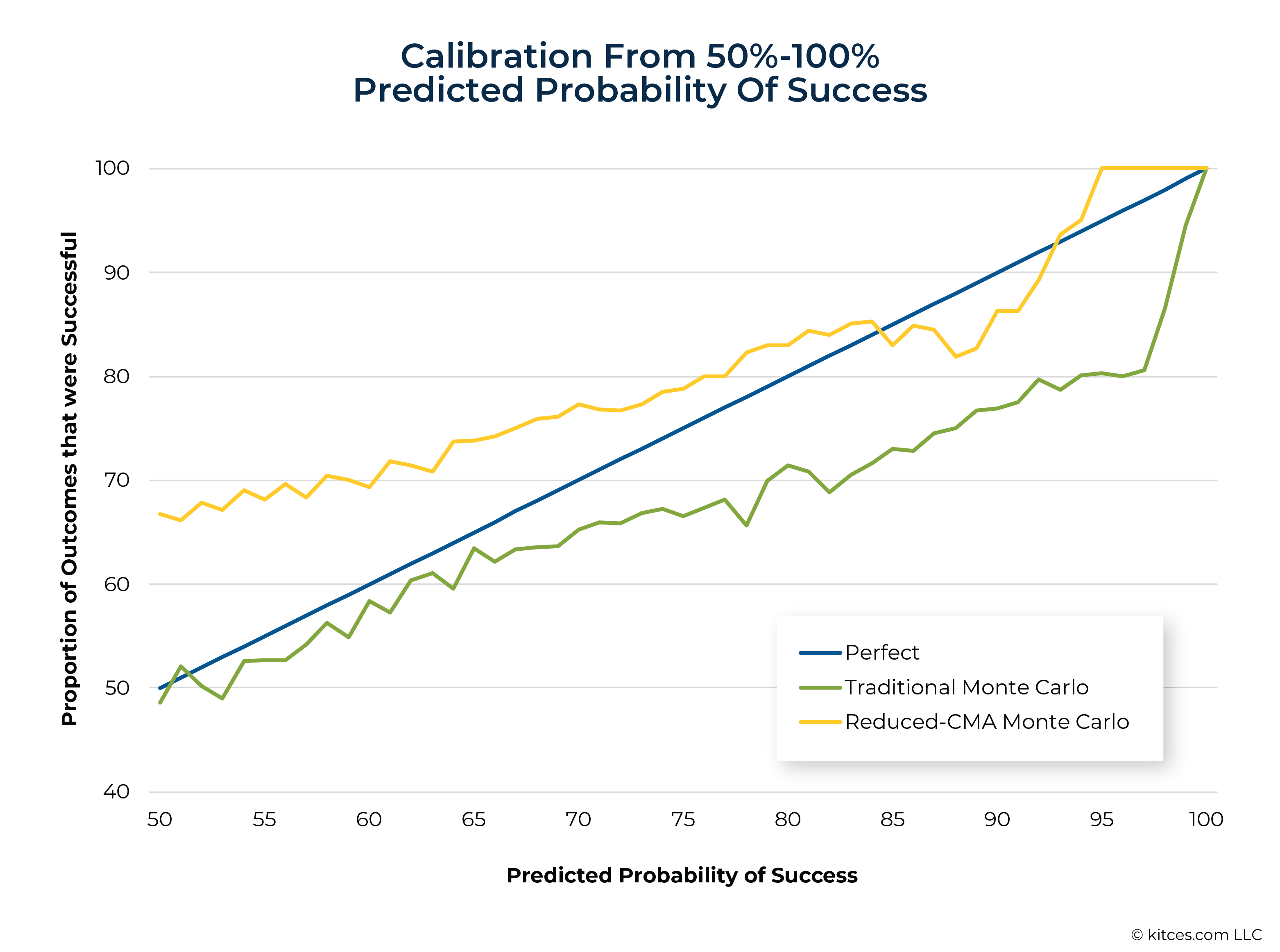
Fortunately, there’s a nice visualization that can help us understand a model’s performance across a range of predictions. We simply plot how often it actually rained for each likelihood level that our model forecasted. A perfectly calibrated model would look like the (blue) diagonal line in the graph below.

If, however, our model systematically over-predicted rain (represented by the yellow line), we’d say it has a “wet bias”. Notably, weather forecasters on your local news often intentionally build in a wet bias to their forecasts. Why? It turns out people are quite happy when they think it’s going to rain but it doesn’t, but they are upset if they don’t think it’s going to rain and then it does. (A model with a “dry bias” is shown by the green line in the graphic above and would underpredict rain, meaning more people would be unhappily caught without an umbrella.)

In practice, we’re unlikely to see perfect calibration, especially for models of complex phenomena. Instead, a model might have a ‘wet bias’ for some probability bands and a ‘dry bias’ for others, or the distance from perfect calibration could vary across the graph. The information on the sizes and types of errors that we see in calibration charts can be helpful in evaluating how much trust we put in probabilistic forecasts – not just for rain, but for financial planning as well.

Forecasting Models In Retirement Income Planning

Financial advisors (and meteorologists) will naturally seek out the best available models to use in forecasting. When an advisor says, “There is an 85% chance that you won’t run out of money if you follow this plan,” this is shorthand for “According to one model of the world, which contains dozens of assumptions but which I believe is reasonable and well-supported, I estimate you have an 85% chance that you won’t run out of money if you follow this plan. There are other models and assumptions I could have used, but I think the approach I used is the best available.”

It is worth asking whether the models that we use in financial planning are indeed reasonable and well-supported, whether there are differences between available ways of producing forecasts, and if there are important biases and miscalibrations to keep in mind when using these forecasts.

We examined the accuracy of probabilistic forecasts of retirement income risk from models of investment returns and inflation. Specifically, we asked how well 4 different approaches to the creation of Capital Market Assumptions (CMAs), return sequences, and inflation sequences perform in the real world.

The assumptions that each model used at each point in history were produced systematically in ways that mirror actual approaches to modeling and CMAs available to and used by advisors today, and are as follows:

1. Traditional Monte Carlo: One set of CMAs applies to all years in the plan: In our analysis of this approach, CMAs that are the average portfolio returns and standard deviation of returns from the preceding 30 years were applied to each point of time examined;
2. Reduced-CMA Monte Carlo: This is similar to Traditional Monte Carlo, except that CMAs are reduced by 2% and standard deviation is reduced proportionally;
3. Historical Analysis: Actual historical sequences of returns and inflation models the range of possible return and inflation sequences. The assumptions for this analysis used all history available up to each point in time; and
4. Regime-Based Monte Carlo: 2 sets of capital market assumptions – one that applies to the near-term and one that applies to the long-term – are used to produce simulated return and inflation sequences. The assumptions exclude half of all prior points from each point in history based on their economic dissimilarity to the point in time being examined. From this filtered set of historical prior points, averages from the first 10 years are used to produce near-term CMAs, and averages from the next 20 years are used to produce long-term CMAs.

To measure the performance of these approaches, we produced probability-of-success forecasts for a range of simple income plans at each point in history from 1951 to 2002. For each historical month, each of these 4 models predicted the probability of success of 200 different income plans (from very safe to very risky). We then compared each predicted probability of success to the actual outcome for that income plan (i.e., did the income plan exhaust the portfolio or not?). This method is analogous to comparing probability-of-rain forecasts to actual observations of rain.

The least familiar of these is likely the Regime-Based Monte Carlo approach. By using multiple sets of CMAs, Regime-Based Monte Carlo is meant to allow advisors to express a view on how returns and inflation may differ over the life of a plan. For example, an advisor who expects lower returns and higher inflation over the near term but reversion to the mean thereafter can reflect these opinions in their analysis. Regime-based approaches have been used in retirement research for over a decade and have been discussed numerous times on this blog. But Regime-Based Monte Carlo has only recently begun to appear in retirement planning software.

In order to produce reasonable Regime-Based CMAs systematically, we used Cyclically Adjusted Price/Earnings (CAPE) ratios, one of many economic factors that can be used profitably to help inform retirement planning, as our measure of economic similarity. So, for example, in 1982, when CAPE was very low, CMAs for Regime-Based Monte Carlo excluded prior scenarios that began when CAPE was very high.

Beyond the methods examined here, there are, of course, other approaches that could be used in producing probability of success forecasts (e.g., accounting for autocorrelation in Monte Carlo simulations or different approaches to producing CMAs), but we’ve tried to focus on methods that are commonly used by and available to advisors in practice. Alternative approaches could have better (or worse) results than those reported here.

Which Model(s) Performed The Best?

We looked at forecasted probabilities of success for inflation-adjusted systematic portfolio withdrawals from a 60/40 stock/bond portfolio over 20 years, where we used 20-year plans instead of the more commonly discussed 30-year plans so that we could examine a wider range of forecast dates through a 2002-2022 retirement (although we also ran this study with 30-year plans and found very similar results). This is a severely simplified ‘retirement income persona’, but one that is useful for research. This same study can and should be done for a wider range of personas.

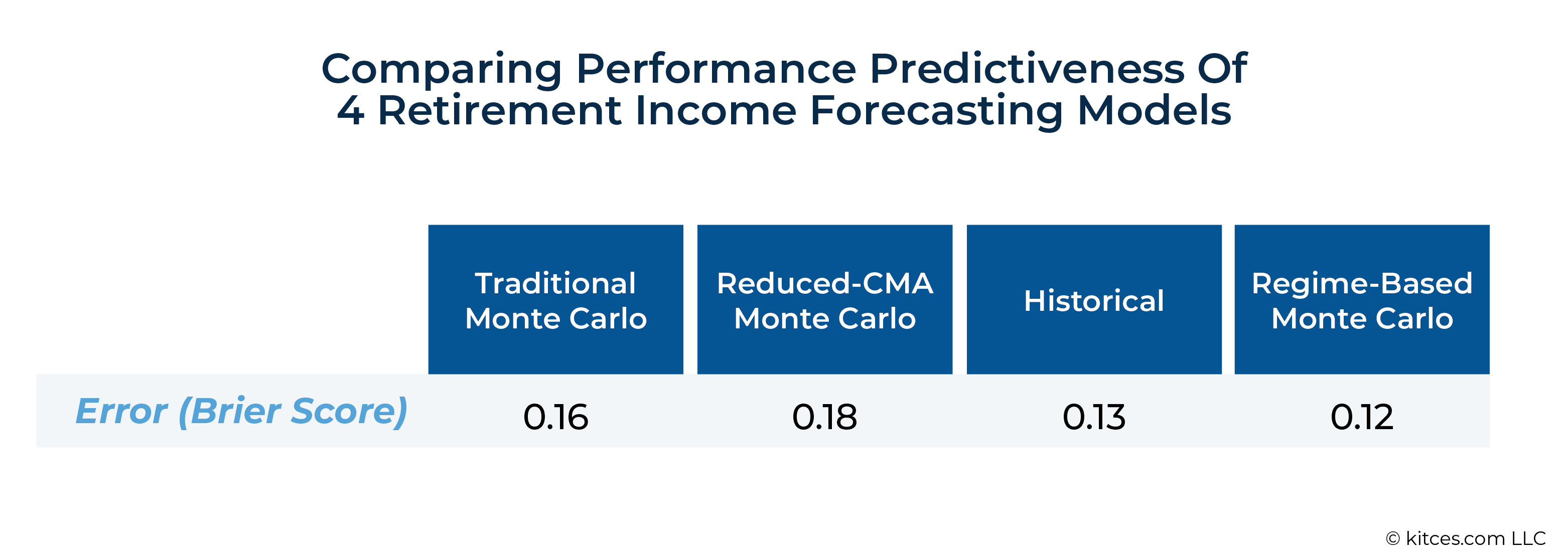
Though all models had significant levels of error, Historical and Regime-Based Monte Carlo analysis significantly outperformed Traditional Monte Carlo and Reduced-CMA Monte Carlo. (For context, a perfect model would have a Brier score of 0. The worst possible Brier score is 1. A model that always forecasts a 50% probability of success for all plans would have a Brier score of 0.25.)

Unfortunately, the poorer-performing methods are far more commonly used in practice than the better-performing approaches. That means that there is plenty of room for improvement in the practice of modeling for retirement income planning.

The Historical and Regime-Based Monte Carlo models had Brier Scores about 25% lower (lower Brier scores are better) than the Traditional Monte Carlo model. The historical model’s good performance may be, at least in part, a reflection of how actual historical market data capture real-world dynamics such as momentum and mean reversion that are not captured in conventional Monte Carlo simulations run by most software programs today. The surprisingly good performance of Regime-Based Monte Carlo CMAs suggests that attention to economic context can also lead to real-world improvements.

But there is more to learn when we examine the calibration of these models.

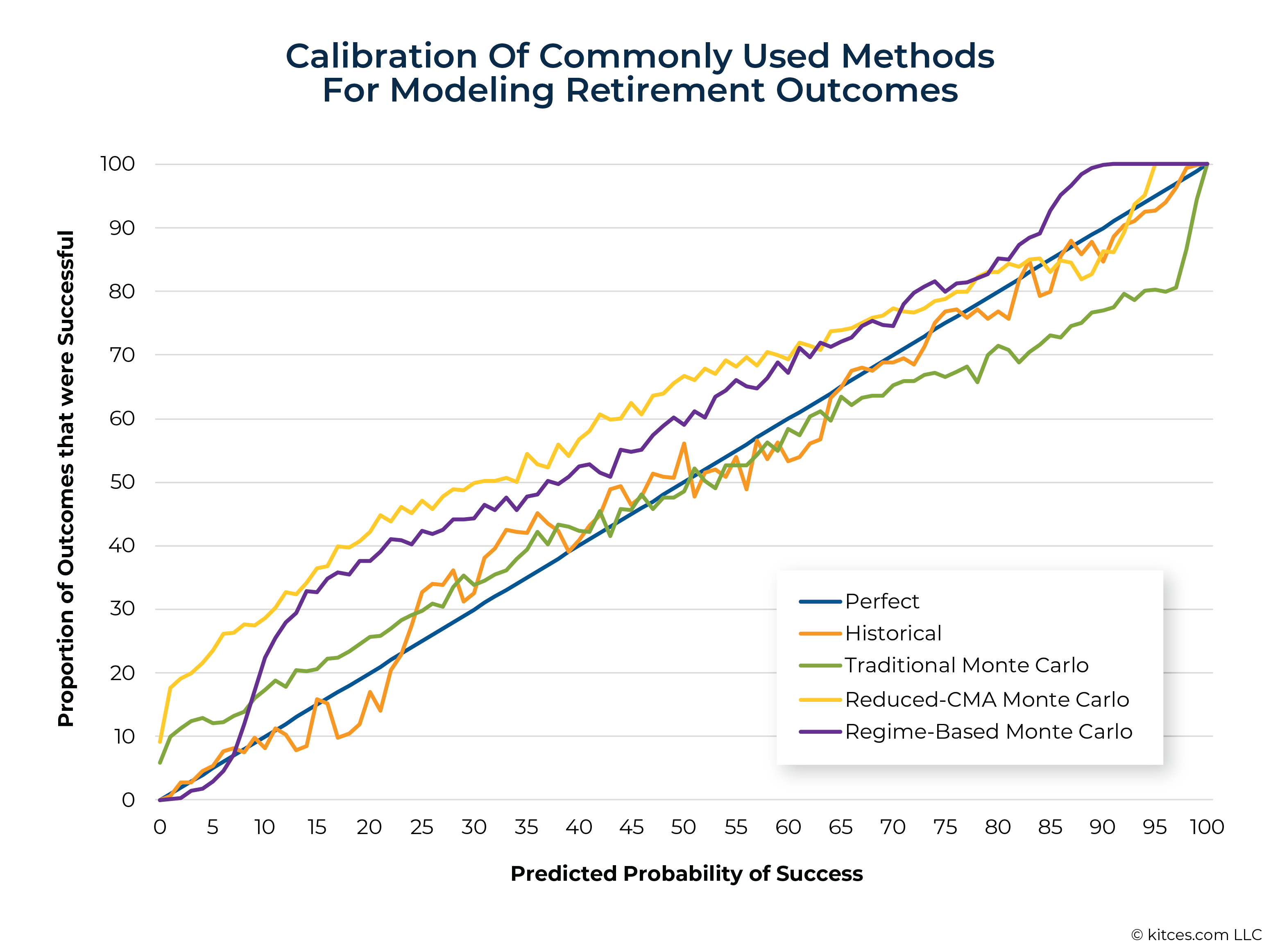
Regime-Based Monte Carlo was one of this study’s best performers, measured by both its very low Brier Score and its calibration, with the best predictions coming at probabilities of success above 60% – exactly the area most important to most advisors. Importantly, Regime-Based Monte Carlo shows a consistent ‘wet bias’: This model tends to predict more metaphorical rain than will really fall. This bias may not be bad in practice, though. Just as pedestrians prefer surprising sun to surprising rain, retirement clients (and their advisors) may prefer unexpected good news. And plans evaluated with Regime-Based Monte Carlo were more likely to turn out better than expected.

The Historical model had a similar Brier Score to Regime-Based Monte Carlo and very tight calibration, especially from 65% to 100% probability of success. However, it did include a mix of miscalibrations, sometimes over- and sometimes under-predicting risk. The Historical model often had a ‘dry bias’ (overconfidence, or an underestimate of risk) above 50% probability of success, but this bias was much smaller than we see for Traditional Monte Carlo.

In fact, the comparatively poor calibration of Traditional Monte Carlo is one of the most important findings of this study. While Traditional Monte Carlo had overly conservative predictions (a ‘wet bias’) below 50% probability of success, it showed marked overconfidence (a ‘dry bias’) above 50%, and particularly between 70% and 97%. What does ‘dry bias’ mean in practice? For every 100 clients who targeted plans with a 95% probability of success using Traditional Monte Carlo, we would have expected 5 of those clients to fail (or, more realistically, to have needed to reduce spending), but instead 20 of them would have found they were spending too much.

A recent survey of financial advisors found that, in practice, advisors generally recommend minimum acceptable probability-of-success levels in the 70% to 95% range. In other words, the errors seen with Traditional Monte Carlo are worst right in the sweet spot of financial advice. Furthermore, this dry bias is more likely to produce unpleasant surprises from overspending. By underestimating risk, this model will tend to lead to income recommendations that are higher than fit given a client’s risk preferences and, accordingly, to more unplanned downward income adjustments in the real world.

This result is notable because one of the most common justifications for the use of Traditional Monte Carlo is that advisors want to model scenarios that could be worse than what we’ve seen historically. In other words, they may believe that Monte Carlo analysis will help them be conservative in their analysis. But, at least based on the approach to Traditional Monte Carlo modeling analyzed here, Monte Carlo simulation was overly aggressive instead of more conservative, at least in the most important half (i.e., above 50%) of the probability-of-success range.

If we zoom in on that area of the chart, we see that predicted probability of success levels were significantly higher than the actual percentage of outcomes that were, in fact, successful.

Though Reduced-CMA Monte Carlo (represented by the yellow line in the graphics above) reduced this dry bias (at the cost of the most extreme wet bias among the candidate approaches), this approach was still overly optimistic from 83%-93% probability of success.

Forecast Accuracy In Different Historical Environments

Due to the constraints of available historical data and our models’ demands for previous historical data to use for constructing assumptions, our study covered just over 50 years of forecasts, from 1951 to 2002 (inclusive). When forecasts are grouped and evaluated in shorter timespans, some of the strengths and weaknesses of these models become clearer.

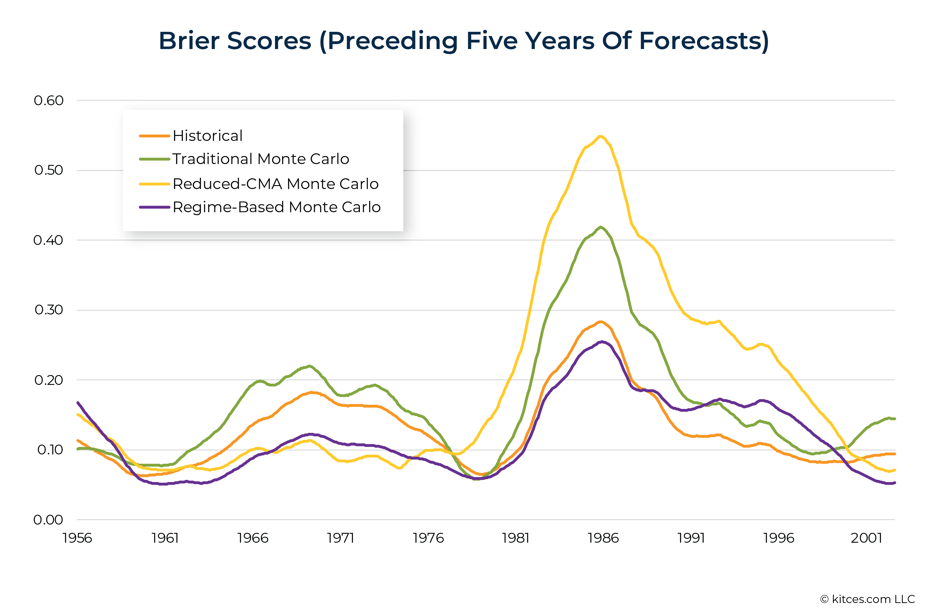
The graph below shows the Brier score for each forecasting approach for each 5-year rolling period. For example, the Brier scores shown at 1986 represents the error level for all forecasts between 1981 and 1986. Historical and Regime-Based Monte Carlo had far lower error (i.e., better forecasts) during that particular 5-year period than did Traditional Monte Carlo or Reduced-CMA Monte Carlo.)

Here we see that Regime-Based modeling almost always had the lowest Brier scores over rolling 5-year periods, indicating that it was almost always the best performer (with Historical often nearby), whether forecasts were made in periods that were good, bad, or middling for retirement income.

The Regime-Based model did very well through the poor inflation-adjusted returns of the late 1960s and 1970s, but was also among the best models (closely matched by Historical analysis) when exiting the stagflation of the 1970s for the boom times of the 1980s when the accuracy of all models suffered. Historical analysis continued to do well through the 1990s and 2000s, while the Regime-Based model performed very well in the Tech Bubble of the early 2000s.

This ability to provide reasonable predictions – no matter what the economic environment is like – is very important. Financial advisors must provide advice in good times and in bad, but it isn’t always clear which we’re living through. In comparison, Reduced-CMA Monte Carlo was a one-trick pony: it only performed well in periods when retirement income turned out, in retrospect, to be under pressure. And because Traditional Monte Carlo used average trailing 30-year returns, it was also a comparatively poor performer (with a few exceptions) because it often found itself “fighting the last war”.

What Is The Best Model To Use In Practice?

Both Brier scores and calibration results suggest that, from the approaches to probabilistic forecasting we examined here, Regime-Based Monte Carlo and Historical models outperform Traditional Monte Carlo and Reduced-CMA Monte Carlo. This outperformance is plausibly due to factors in the better-performing models that simply match the real world more closely and allow for more precise forecasts in any economic environment. Therefore, advisors and clients who can access better models can reasonably expect to produce better advice.

This is not to say that any of the models we’ve discussed approach perfection. On the contrary, another takeaway is that all models’ predictions are rife with errors. Brier scores were never 0 or even close to 0 for any approach. This should humble any forecaster. Advisors should be aware of both the likelihood of error in general and the nature of these errors specifically.

For example, when using Regime-Based Monte Carlo, advisors should keep in mind that this model’s predictions consistently erred on the side of caution, predicting lower probability of success than what actually materialized. Of course, this bias isn’t necessarily a bad thing since it matches client and advisor preferences for positive surprises. Advisors who don’t or can’t access more accurate models should also understand the pitfalls of Traditional Monte Carlo and possibly correct for this shortcoming by targeting higher probabilities of success than they would otherwise have sought in order to avoid  overconfidence.

It is also worth noting that advisors might want to consider different models based on the goal of their modeling. Based on the results here, an advisor trying to develop a ‘best guess’ might lean toward a historical model, whereas an advisor trying to build in some risk aversion might lean toward a Regime-Based Monte Carlo approach. Moreover, using a blend of different approaches and ‘triangulating’ on a result may be worth considering, as well. Most planning software programs don’t offer multiple forecasting models, and instead focus on just Traditional Monte Carlo. To the best of our knowledge, Income Lab, which both of us are affiliated with, is the only tool that currently can handle Traditional Monte Carlo, Regime-Based Monte Carlo, and Historical simulations. However, that will hopefully change as more tools begin to offer greater diversity of forecasting models.

Since errors in forecasts are a near certainty, these results also provide an additional reason to plan for adjustments to retirement income. As time goes on, advisors and clients learn more about the world they are living in and can make adjustments to counteract some of the errors that crept into their initial analyses. Failing to have a process for updating forecasts over time would be like making a weather forecast a week out and then failing to watch the sky and the radar as the days go on. If clouds are forming and the radar is green, the probability of rain has gone up and we can batten down the hatches if need be. If the sky and radar are clear, the probability of rain has gone down and we can get ready to enjoy smoother sailing.

A responsible advisor will, of course, try to use the best forecasting models available, but they also won’t stop checking the sky and adjusting their advice if need be.