Executive Summary
Financial advisors often rely on software that uses Monte Carlo simulations to incorporate uncertainty into their retirement income analysis for clients. While Monte Carlo analysis can be a useful tool to examine multiple iterations of potential market returns to forecast how often a given plan may be expected to provide sufficient income for the client throughout their life, there is a lot about Monte Carlo simulation that we are still learning. For instance, advisors may wonder if there is any benefit to increasing the number of Monte Carlo scenarios in their analyses to provide a more accurate picture of the range of potential sequences of returns a client might face.
While financial planning software typically uses 1,000 scenarios, advances in computing make it possible to run 100,000 or even more scenarios within reasonable amounts of time. To examine the potential impact of various numbers of simulated scenarios that could be chosen, we tested how consistent Monte Carlo plan results are when run at different scenario counts and iterated these simulations 100 different times. We find that the variation of sustainable real annual retirement income suggested by simulations running 250 versus 100,000 scenarios varies only by about 1.5% for given levels of spending risk. However, the variation is wider at the extreme tails (0% and 100% risk), which provides some particular considerations for those who might be aiming for as close to 100% probability of success as possible. Ultimately, the results of our first analysis suggest that the common scenario count levels built into Monte Carlo tools today are likely to be adequate to analyze the risk of different spending levels.
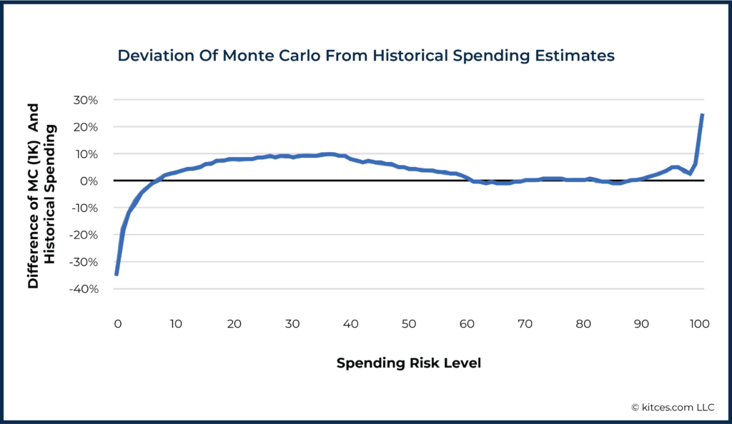
Another common concern is how Monte Carlo results might differ from historical simulations. Monte Carlo results are often considered to be more conservative than historical simulations – particularly in the US, where our limited market history contains the rise of the US as a global economic power. In our analyses, we find that the two methods provide differing results in a few notable areas. First, Monte Carlo estimates of sustainable income were significantly lower than income based on historical returns for the worst sequences of returns in the simulations (which give us risk spending levels of 0–4/96–100% probability of success). In other words, Monte Carlo results projected outcomes in extreme negative scenarios that are far worse than any series of returns that have occurred in the past. Similarly, for the best sequences of returns in the simulations, Monte Carlo suggested sustainable income amounts significantly higher than historically experienced (corresponding to spending risk levels of 88–100/probability of success 0–12%). Both results are possibly due to the treatment of returns in consecutive years by Monte Carlo as independent from each other, whereas historical returns have not been independent and do tend to revert to the mean.
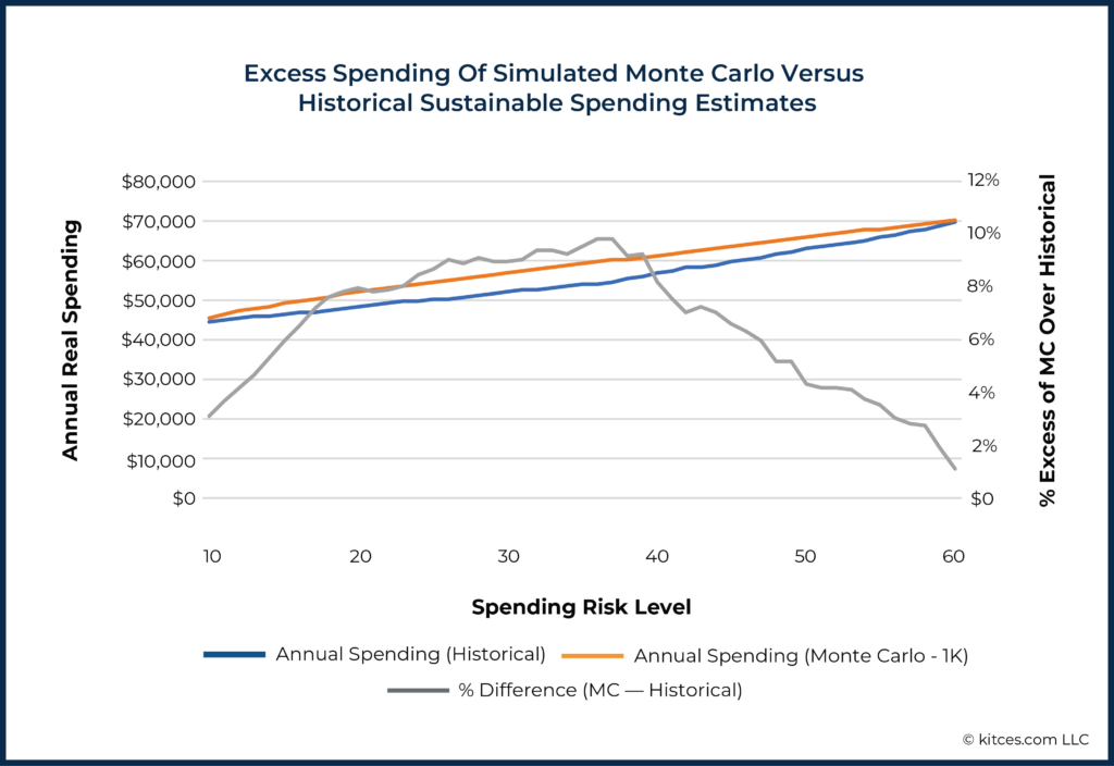
Interestingly, Monte Carlo simulations and historical data also diverged at more moderate levels of risk (spending risk levels of 10–60/90–40% probability of success), with Monte Carlo estimating 5–10% more income at each risk level than was historically the case. Which means that, rather than Monte Carlo being more conservative than historical simulation as commonly believed, at common levels used for Monte Carlo simulation (e.g., 70% to 90% probability of success), Monte Carlo simulations might tend to be less conservative compared to historical returns! One way advisors can address this issue is to examine a combination of traditional Monte Carlo, regime-based Monte Carlo (where assumed return rates differ in the short run and the long run but average out to historical norms), and historical simulation to explore a broader range of potential outcomes and triangulate on a recommendation accordingly.
Ultimately, the key point is that while future returns are unknowable, analytic methods such as Monte Carlo and the use of historical returns can both provide advisors more confidence that their clients’ retirement spending will be sustainable. Contrary to popular belief, Monte Carlo simulation can actually be less conservative than historical simulation at levels commonly used in practice. And while current financial planning software generally provides an adequate number of Monte Carlo scenarios, the deviation from historical returns at particular spending risk levels provides some additional insight into why multiple perspectives may be useful for informing retirement income decisions. Which suggests that incorporating tools that use a range of simulation types and data could provide more realistic spending recommendations for clients!
Financial planning software programs that use simulation analysis typically depend on Monte Carlo methods. At their core, these methods involve exploring many possible scenarios of market returns to discover how a client’s retirement spending plan would play out in those scenarios.
Typically, most software systems use 1,000 scenarios, but in some cases, they may use as few as 250. Choosing the number of scenarios was usually based on the assumption that using “a lot of scenarios to average out and understand the health of the client’s plan” provided a robust assessment, but was balanced against the technology constraint that doing a larger number of scenarios often meant sitting an uncomfortably long time just waiting for the software to run. As computer processing speeds have improved, though, we might ask whether it would be better to use 2,500, 5,000, 10,000, or even 100,000 or more scenarios now that it is more feasible to do so.
The question becomes one of examining what is gained and lost in the arena of retirement income planning as we change the number of scenarios used in each Monte Carlo simulation. Will the estimated risk levels of various incomes change as we rerun Monte Carlo simulations? Do the results of a smaller number of simulations differ markedly from a simulation with more scenarios? And how do Monte Carlo results compare to other simulation methods, such as the use of historical return sequences?
These questions are not just idle mathematical musings – they have real import for the practice of financial planning when any sort of simulation method is used, where advisors make recommendations to clients on the basis of the outcome of that analysis or projection.
In order to explore these questions, we make use of a concept introduced in a recent article – the spending risk curve.
Spending Risk Curves
Simulation methods in financial planning help us incorporate uncertainty into our thinking, as we may have a belief of how returns will average out in the long run, but we don’t necessarily know how it will play out in any particular sequence (which is important, given the impact of sequence of return risk!).
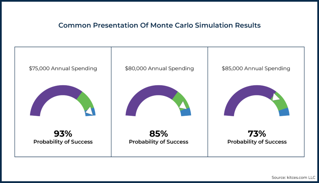
To address this challenge, it is common to use simulation analysis to explore the likelihood that a given income plan will exhaust financial resources before the end of a defined period, providing an understanding of the level of risk that such an income goal entails. The results of this focused question are often expressed as a probability of success (or probability of failure) and visualized with a dial or similar figure.
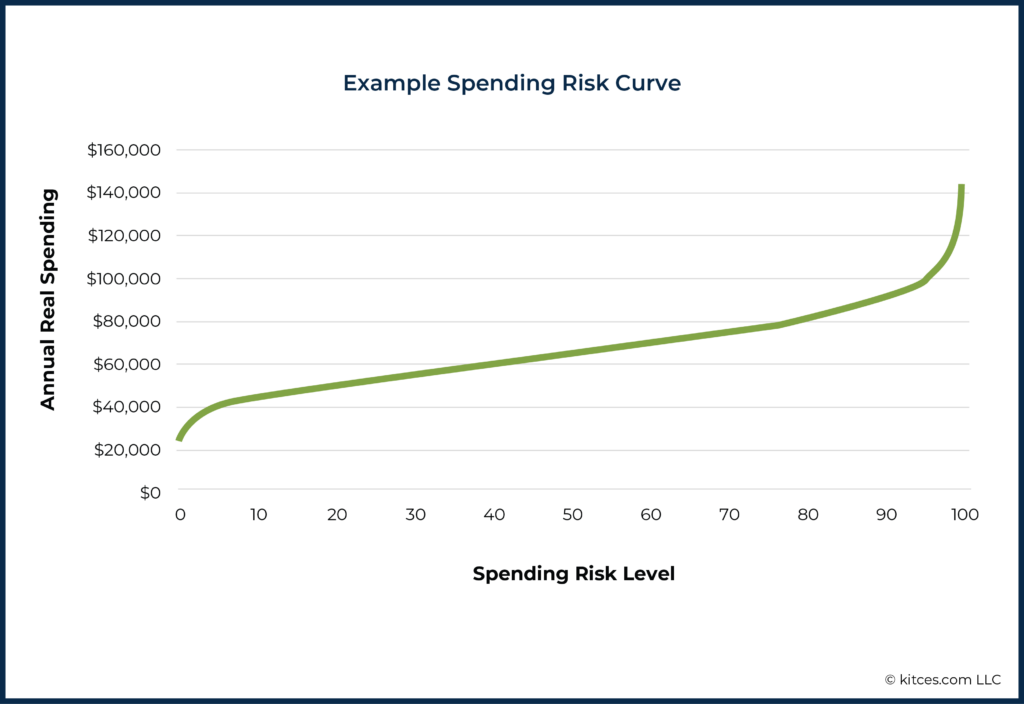
However, this approach is too narrow for understanding the broader relationship between income levels and risk levels, especially since our brains are not naturally wired to think probabilistically about the relative safety of a single particular retirement income goal. Instead, using technology, it is possible to develop figures that show the retirement spending that can be achieved at any risk level or, vice versa, the risk of any spending level, which makes it possible to consider risk, not in a binary manner (is the probability of success for this goal acceptable or not?) but instead over a range of outcomes (given the risk-return trade-offs along the spectrum, what is a comfortable balancing point for me?).
For example, the following shows the (inflation-adjusted) portfolio withdrawals that would be available from a $1 million 60/40 portfolio over 30 years based on a Monte Carlo analysis. For our capital market assumptions, we use the mean monthly real return (0.5%) and monthly standard deviation of returns (3.1%) from a 60/40 portfolio over the last 150 years. Crucially, this is the same historical data we will use below when discussing historical simulation.
The end result is something more akin to an efficient frontier in the investment risk-return trade-off for a portfolio, except in this context, it is a spending risk-return trade-off instead.
Notably, along with many others, we have argued elsewhere that framing risk as “failure” (as in the success/failure paradigm common in Monte Carlo systems) is both inaccurate (retirees do not typically fail – they adjust) and can lead to unnecessarily heightened fear and anxiety. As a result, it is a conscious decision to use the more neutral “spending risk” term here.
Spending risk (1 minus the probability of success) can be thought of as the estimated chance that a given income level will not be sustainable at that constant level through the end of the plan and, therefore, that a downward adjustment will be needed at some point before the end of the plan to avoid depleting the portfolio (which means the retiree never spends until they run out of money at the risk of destitution; it’s simply a question of whether their spending sustains or experiences a pullback).
How Do Monte Carlo Results Vary By Number Of Scenarios?
Many popular planning software systems use 1,000 scenarios in their Monte Carlo simulations, but there is some variation in the market. Furthermore, financial advisors might wonder whether the number of simulations offered in commercial software gives the simulations enough power to be depended on. Would a larger simulation deliver different results?
In order to explore these questions, we ran 360-month (30-year) Monte Carlo simulations with 250, 1,000, 2,500, 5,000, 10k, and 100k scenarios, using a $1 million 60/40 stock/bond portfolio. For each tier of the number of scenarios (250, 1,000, 2,500, etc.), we ran the simulation 100 times to see how much the results varied with repeated ‘simulation runs’ while keeping the number of scenarios within each of the simulation tiers constant.
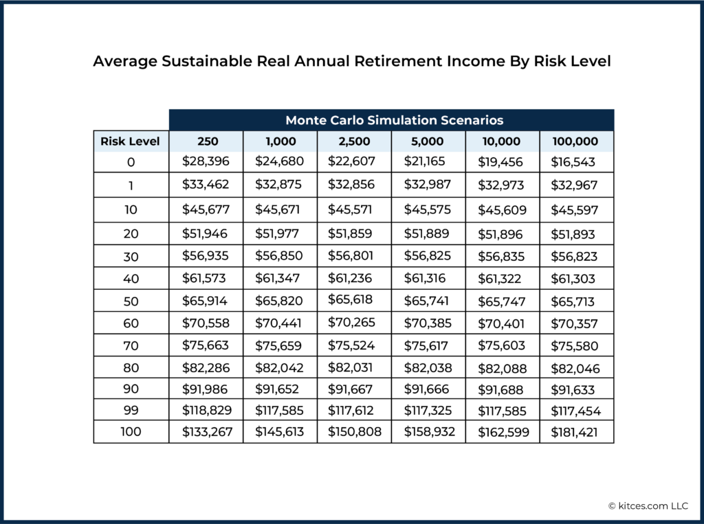
The averages (means) of the amount of sustainable real annual retirement income found at each decile of risk for each set of 100 simulations are shown in the table below. (We’ve also included values for both the ends of the risk spectrum - 0 and 100 - and one point up the tails - 1 and 99 - in preparation for further discussion of these extremes below.)
We immediately see that only the minimum and maximum risk levels (0 and 100) show unacceptably large variation as we change the number of scenarios in the Monte Carlo simulations. We will return to these extremes of the risk spectrum below and discuss how the tips of the tails of the spending curve for Monte Carlo analyses can be problematic.
In the middle 80% of the risk spectrum (i.e., Risk Levels between 10 – 90), these results show a 0.4% or less difference between the 100,000-scenario Monte Carlo and the much smaller 250-scenario simulations. (And even the 1 and 99 levels only show differences in the 1.5% range – levels that might be acceptable for all practical purposes.)
In other words, the mean results do not differ appreciably depending on the number of scenarios in the Monte Carlo analysis. By this measure, running additional scenarios doesn’t yield any advantages. But, before we conclude that a 250-scenario simulation will be just as good as a 100,000-scenario test, we need to ask how much these results fluctuate around the mean with each successive run of the simulation.
After all, Monte Carlo methods typically involve the randomization of returns. If this randomization results in very little fluctuation, each simulation will be consistent with the last. But if there is broad variation, we might conclude that we are using too few scenarios in our simulation to derive high confidence from a single simulation run.
In other words, just because the average of the spending found at each risk level across 100 simulations of 250 scenarios is similar to the average spending levels found across 100 simulations of 100,000 scenarios each, it doesn’t mean any particular run of 250 simulations won’t differ significantly from any particular run of 100,000 scenarios or will be representative of the ‘true’ simulated values.
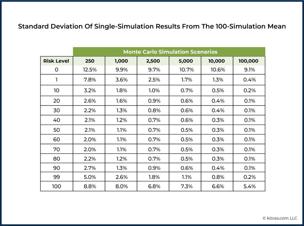
Standard deviations of the spending levels (expressed as a percentage deviation from the mean result) are shown below. As we might expect, inter-simulation variability of spending levels drops as we add scenarios to the simulations.
Even relatively sparse 250-scenario simulations keep inter-run variability (as measured by standard deviation) within a reasonable 2-3% range when avoiding the extremes of the risk spectrum. This level of variability is well within what we might expect for actual spending variation in real life. After all, clients will rarely – if ever – spend exactly as specified in their retirement plan (vacations will be altered or canceled; unexpected home repairs will arise). The common 1,000-scenario simulation keeps us in a barely-observable 1-2% range.
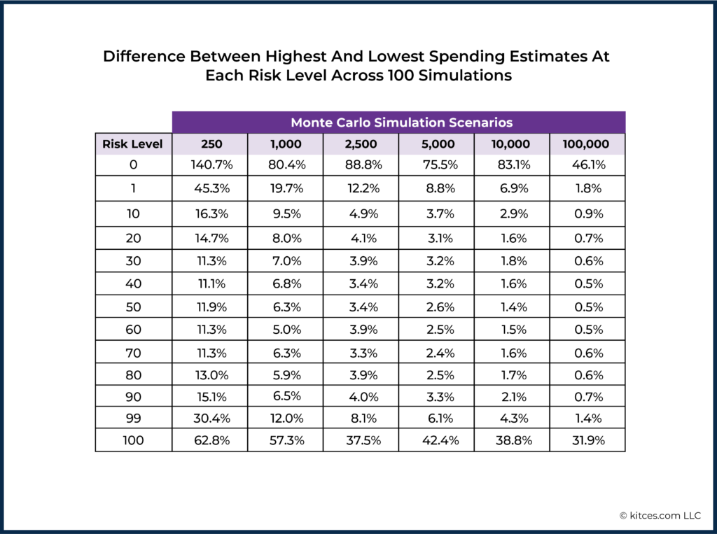
In more practical terms, it can be confusing and discomfiting for planners and clients to see large changes in a plan’s results upon repeated analysis, even if no changes have been made! The largest difference between any two simulations’ estimated spending at each risk level is shown below. This measures how much larger, in the extreme, spending estimates could be from one run to the next. This means that, in the worst case, we might expect a $100,000/year spending level at a risk of 10 to become $110,000/year when we rerun a 1,000-scenario simulation. Such a sudden shift from one simulation to the next should be extremely rare, but, armed with this data, advisors can know how much results might vary when running many simulations of the same plan.
Deciding the ‘right’ number of scenarios for Monte Carlo simulations is a practical matter and a judgment call, and advisors may differ on that judgment. However, the results in this section suggest that, when ignoring the extremes of the risk spectrum, the status quo is hard to criticize, and there is little need for more powerful, higher-scenario-count Monte Carlo simulations for retirement income planning.
We’ve also seen evidence here that the edges of the distribution (extremely low risk and extremely high risk) show both large differences when comparing simulations with different numbers of scenarios and high inter-simulation variation when keeping scenario counts constant. We’ll now take a closer look at these extremes.
What About The Tails?
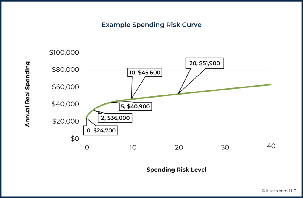
Using spending risk curves to evaluate retirement planning options helps advisors understand the cost/benefit trade-offs between higher/lower annual real retirement spending and higher/lower spending risk levels.
There's a lot that we can quickly glean from the shape of such a curve for a given plan. For instance, the curve above highlights just how dramatically spending falls off for those trying to achieve that last 10% in their probability of success – while going from a risk level of 10 to a risk level of 20 (equivalent to moving from 90% probability of success to 80%) increases spending by 14% from $45,600 to $51,900, moving from a spending risk level of 10 to a risk level of 2 cuts spending down by 27% to $36,000/year. Those insisting on 100% success would have to accept $24,700/year according to this curve!
Given the high potential cost in standards of living that would have to be paid in order to achieve these low risk levels, it is important to know whether these Monte Carlo results are to be trusted. We’ll first look at these ‘lower tail’ results as we did above – by looking at how results differ when we add or subtract scenarios from the simulation and by examining inter-simulation variation. In the next section, we’ll see how Monte Carlo results compare to historical simulations.
The lower end of the risk spectrum (0-9% chance of failure, or, equivalently, 91-100% chance of success) is generally where, anecdotally, we have found that advisors – and clients – often want their financial plans to land.
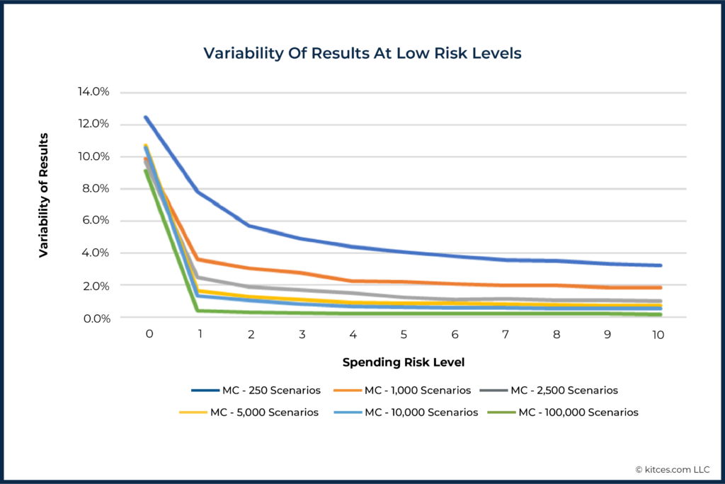
The graph below shows how much the estimated income for these low risk levels (i.e., the 10th percentile, 9th percentile, 8th percentile, etc., all the way down to the 2nd, 1st, and 0th percentiles) varied across 100 runs of each type of Monte Carlo simulation.
We can conclude at least two things from this picture. First, the 250-scenario Monte Carlo simulation has a very high inter-run variability as the lowest risk levels – close to or higher than 4% and, in the extreme, above 12%. The analyses with at least 1,000+ simulations differed far less across runs, to the extent that ‘just’ going from 250 to 1,000 simulations cuts the variability by almost as much as going from 1,000 to 100,000!
However, the results also highlight that all types of Monte Carlo analyses suffered from a much higher variability at the extreme 100% success/0 spending risk level. That’s because this is literally the worst scenario in the simulation, and differences in exactly how this worst scenario plays out in repeated simulations are bound to be higher than in the ‘thicker’ parts of the distribution of results.
In the case of the true extremes – literally, the last 1% of results – there is nearly always at least one unusually extreme scenario somewhere in the Monte Carlo simulations. However, with at least 1,000 scenarios, variability immediately drops below 4% of income for the other 99% of results and approaches 2% variability for the remaining 96% results (i.e., beyond the 4% most extreme results).
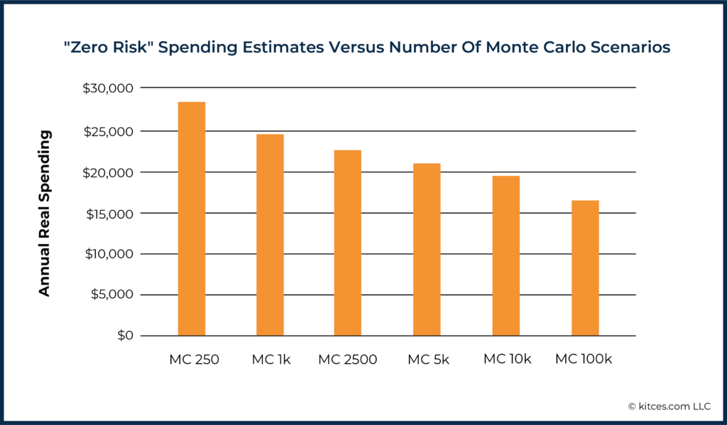
At the same time, it’s also important to recall that not only does the variability of results differ at low risk levels, but at the extreme 0% risk level, the means (i.e., average income that can be sustained in the first place) among these Monte Carlo types differ as well, as we saw earlier.
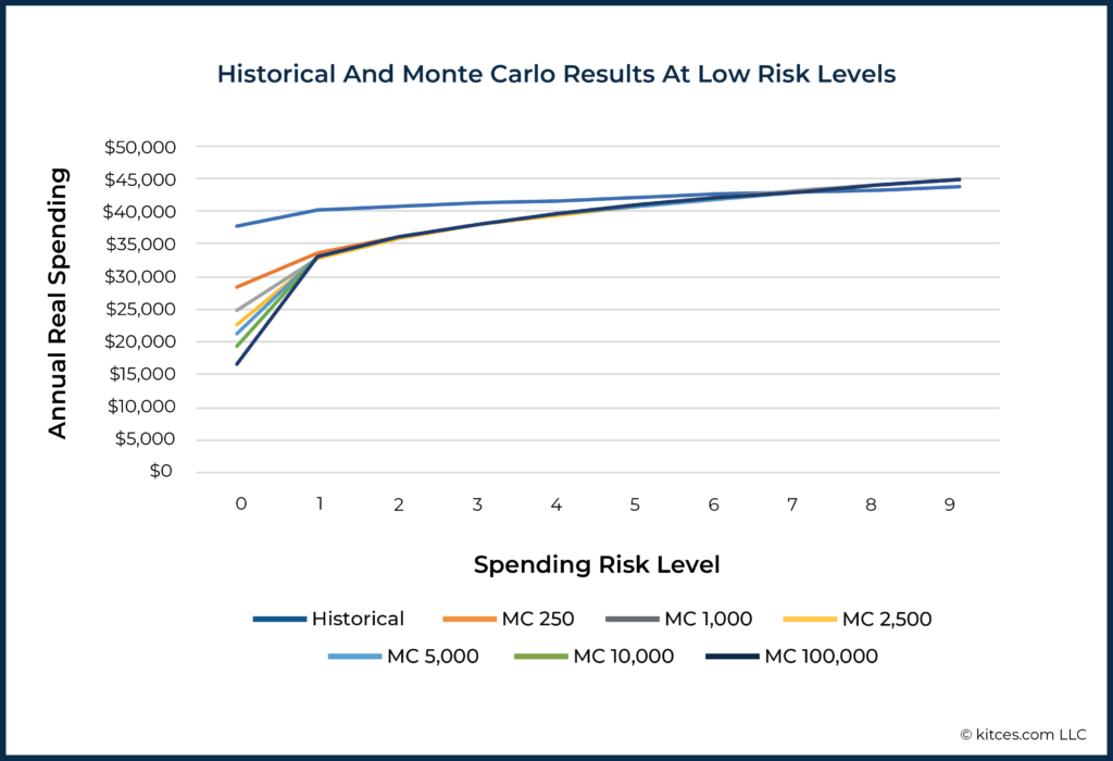
Here the 100,000-scenario simulation sees a $16,540/year spending as being ‘risk-free’ (literally, it didn’t fail in any of the 100,000 simulations), while the 250-scenario simulation would allow almost $1,000/month more at the same risk level. So, while a 250-scenario Monte Carlo has higher variability in this extreme than, say, a 100,000-scenario simulation, the mean result for this risk level is much less extreme for a 250-scenario simulation than we see for simulations with higher numbers of scenarios. In other words, the more scenarios we have in our simulation, the more extreme the result for extreme risk level gets.
These results should give advisors pause. Given that the framing of probability of success can gamify behavior and lead clients to seek ‘maximum’ probability of success, those who follow this incentive too far could be forced to reduce their standards of living significantly in order to gain the very last point on their probability of success meter.
Of more concern, though, is that given the patterns we just discussed, the values we see for 0% risk appear more likely to be artifacts of the simulation methodology, not true facts about the world. After all, it is in the nature of Monte Carlo simulations to include some scenarios where sequences of returns are incredibly poor or incredibly favorable. The more randomized trials we run (as in the 100,000-scenario simulation), the more likely it is that we see many years or decades of poor returns, with little or no reversion to the mean.
In other words, in the real world, at some point when the market drops 40% for 3 years in a row, stocks get so cheap that a rebound is much more likely. But as typically modeled in a Monte Carlo simulation, each given year has an equal likelihood of a crash, whether it follows three years of large market losses or not. Such scenarios won’t be common, but they are more likely to occur at least once in a larger simulation.
Many advisors may already be of the opinion that a 98% or even 95% probability of success is close enough to 100% to be interpreted as essentially ‘risk-free’. The results shown here suggest that treating very low risk levels in Monte Carlo with suspicion may well be warranted.
In order to examine how trustworthy the results of Monte Carlo simulations are outside of the risk extremes, we need to ask another question, which we’ll turn to now.
Worries About Historical Simulations For Retirement Projections
Though a lot of foundational work on retirement income planning has been done using historical analysis, this simulation method is not widely available in commercial software. While there may be many reasons for this, one is surely the worry that using history alone will weaken the plan’s analysis or will not provide a wide enough range of scenarios in which to evaluate a plan.
First, the challenge is that ‘only’ having a century and a half of data, relative to the seemingly unlimited range of potential futures that could occur, raises the concern that we just don’t have enough historical scenarios to model much. After all, as noted earlier, even ‘just’ 250 Monte Carlo scenarios produce relatively high variability of results, and at best, there are only about 150 years of historical data that we can use for historical simulations.
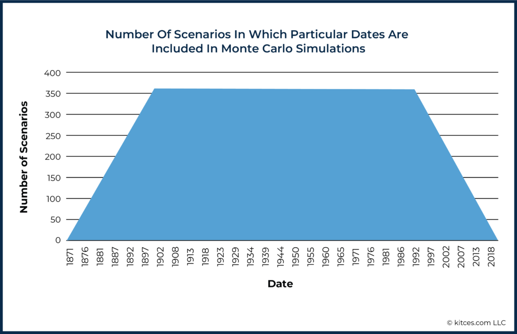
Second, many have argued that within the set of available historical return sequences, there are even fewer independent sequences. Instead, there is wide overlap among scenarios. For example, if, at best, we have about 1,800 months (150 years, beginning in 1871) of data, most of these months are included in 360 (overlapping) scenarios for a 360-month (30-year) retirement plan projection.
The end result of these dynamics is the concern that the level of overlap of dates that occur in historical scenarios weakens the analysis and/or whether using historical models could exclude consideration of scenarios that might occur in the future but have not occurred in the past. All of which could lead to an overly rosy model of the future based on historical analysis alone. In other words, advisors may wonder if historical analyses will lead them to recommend income levels that are too high, or to underplay the risk of a given income plan.
These worries would be valid when they have a real-world effect on planning, and the spending risk curve highlights the place where simulations make contact with real-world decision-making. After all, it is risk – whether expressed as “probability of success”, “chance of adjustment”, or just “spending risk” – that drives many retirement-income-planning decisions. So, we can use the spending risk curve to test whether (and how) historical simulations differ from Monte Carlo simulations, and whether worries about potential inadequacies or weaknesses with historical analysis are warranted.
To be clear, the worry is that historical analysis might overstate income or understate risk. We will see below that quite the opposite is true for the usual range of risks that advisors seek when developing plans.
In other words, when Monte Carlo and historical simulations are compared apples to apples, it is Monte Carlo simulations that seem to understate risk, at least for a core part of the risk spectrum.
Do Monte Carlo Results Match Historically Available Retirement Spending Projections?
Though the future need not repeat the past, and past performance is certainly no guarantee of future results, we can ask about the real spending levels we find at each spending risk level when spending and spending risk are measured using historical return sequences. We can then use these results to see whether spending and spending risk, as estimated through Monte Carlo methods, matches historical patterns.
Again, we took 360-month retirement periods using a $1 million 60/40 stock/bond portfolio and found the real spending levels that would have failed 0%, 1%, 2%, etc., of the time since 1871. These roughly 150 years give us over 1,400 rolling 30-year retirement periods to examine, with a different retirement sequence beginning in each historical month (e.g., starting in January 1871, in February 1871, in March 1871, etc., all the way out to October of 1991, November of 1991, and December of 1991 (for 30-year retirements that finished by the end of available data in March 2022).
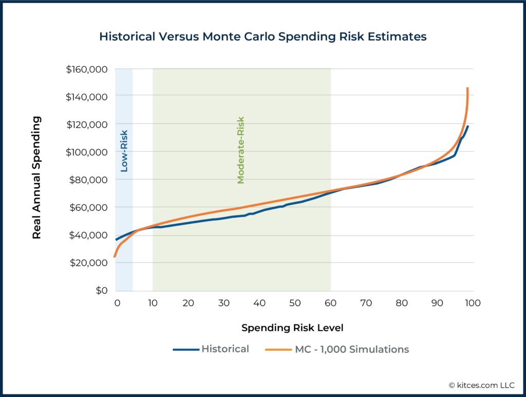
The historical spending risk curve has a familiar shape, but there are some notable diversions from the values we saw for the 1,000-scenario Monte Carlo simulation, as shown below.
Focusing on the lower half of the risk curve, there are two zones in which Monte Carlo results differ markedly from historical patterns:
- The ‘Low-Risk’ Zone (Income Risk Levels 0 to 4): Monte Carlo estimates that spending needs to be reduced drastically below historically low-risk spending levels in order to attain low risk. (In other words, Monte Carlo is actually projecting outcomes in extreme negative scenarios that are far worse than anything that has ever occurred)
- The ‘Moderate-Risk’ Zone (Income Risk Levels 10 to 60): Monte Carlo estimates that 5-10% more income is available at each risk level than was true historically (i.e., Monte Carlo is anticipating less risk in ‘moderately bad’ scenarios than there actually has been when markets have had multi-year runs of poor returns.)
Focusing even further again on the lowest end of the risk spectrum, we notice at least two things:
- All Monte Carlo ‘zero-risk’ incomes lag significantly below the income that has never failed historically ($3,138/month); and
- the more scenarios in the simulation, the worse this deviation is.
In other words, the greater the number of scenarios in the Monte Carlo simulation, the more Monte Carlo projections come up with 1-in-100 (or 1-in-1,000, or 1-in-100,000) events that have never occurred historically but can still be produced by a Monte Carlo random number generator.
It might be tempting to view this information as evidence that historical data does not provide a wide enough range of scenarios and that, at this low end of the risk scale, Monte Carlo analyses may be a more conservative method for modeling retirement projections. This may be true. However, it has been noted that the tails of the Monte Carlo simulation are subject to what are arguably unrealistic extremes.
In particular, it is worth considering that real-world markets tend to be mean-reverting, whereas Monte Carlo simulation generally is not. The tail outcomes of Monte Carlo simulations with a large number of scenarios are going to reflect very extreme scenarios.
For instance, suppose, by pure chance, a Monte Carlo simulation results in 10 straight years of negative returns. In the real world, after such a prolonged bear market, valuations would be low, dividend yields would be much higher, and forward-looking 10-year return expectations would likely be higher than average, none of which is considered by traditional Monte Carlo projections. Therefore, it might be just as plausible that this difference between Monte Carlo and historical results at the extremes is not a feature of Monte Carlo but a bug.
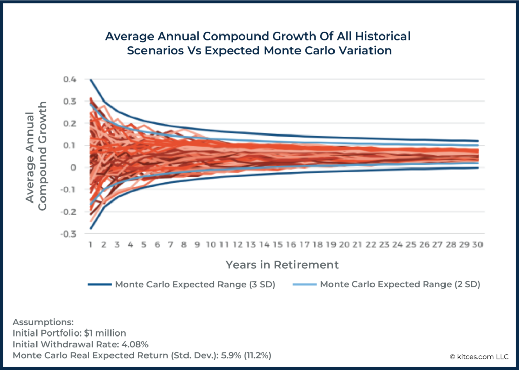
We see evidence of both momentum (short-term) and mean reversion (long-term) when we look at real-world data. Or, to put it differently, returns in the real world are not fully independent of one another. There is a negative serial correlation in market cycles (as prolonged bear markets turn into long(er)-recovering bull markets) that Monte Carlo typically fails to consider.
This is captured well in the graphic below, which shows that in the short-term, historical sequences are outside of the 2 standard deviation level more than we would anticipate (momentum), whereas, in the long run, historical sequences are actually more tightly constrained than we would anticipate, with scenarios not occurring outside of the 2 standard deviation level (mean reversion).
Second, in the ‘moderate’ range of the risk curve with spending risk levels from 10 to 60, Monte Carlo methods overshoot the historical patterns of sustainable spending by as much as 10% at some points.
As an example, the Monte Carlo simulation estimates that spending of $52,000/year has a spending risk level of 20 (i.e., an 80% chance of success). But the historical analysis says that this spending level would have a risk level of 30 (70% chance of success). We do not know, of course, which of these estimates is correct about the still-unknown future (if indeed either is correct). But it is worth highlighting that, in this case, the Monte Carlo analysis is the more aggressive of the two simulation methods. If the historical simulation is more accurate, Monte Carlo may be underestimating risk in this case by as much as 10 points (ostensibly because, as noted earlier, Monte Carlo fails to consider short-to-intermediate-term momentum effects).
It is notable that in exactly the risk range most preferred by advisors (10-40 spending risk level; 60-90% probability of success), Monte Carlo analysis provides higher income estimates/lower risk estimates than historical simulation. This is the reverse of the worry that many may have about using history as a model of the future: it turns out that, in the typical range of outcomes that advisors focus on, history is actually the more conservative approach!
Thus, while it may be prudent not to be overly tied to historical returns and specific historical sequences, many will (or, at least, should?) feel uncomfortable using Monte Carlo projections that effectively assume income risk will be lower in the future than it was already demonstrated to be in the past (or, equivalently, that the income available at a given risk level will be higher going forward than it actually was in the past).
Looking at the upper half of the risk spectrum and focusing on the commonly used 1,000-scenario Monte Carlo simulation, we see the following when compared to historical patterns.
- Moderate/High Risk: Monte Carlo and historical incomes roughly coincide from 60% to 87% risk
- Extreme risk: Starting at about 88% chance of failure (12% chance of success), Monte Carlo results begin to exceed historical incomes, eventually by large amounts. As with the low end of the risk spectrum, this is likely due to the tendency of Monte Carlo methods to overstate the tails.
In summary, we can look at the differences between Monte Carlo and historical simulations across the full risk spectrum.
Note in earlier illustrations that Monte Carlo simulations with different numbers of scenarios differ only at the extremes from this 1,000-scenario pattern. All Monte Carlo simulations showed the same pattern at Low/Moderate and Moderate/High risk levels when compared to historical returns.
Using Historical Returns As A Viable Alternative To Monte Carlo
Ultimately, the data suggest that historical return sequences really are viable alternatives to Monte Carlo: to the extent that we anticipate the range of future outcomes to at least be similar to the range of both good and bad scenarios of the past, Monte Carlo methods appear to overstate the income available at commonly used risk levels, and understate the income available at the lowest risk levels. And if the future is worse than the past, then this problem would be exacerbated: historical simulation would still be the more conservative of the two approaches.
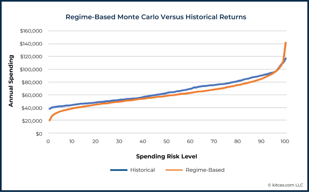
While less commonly available in commercial software, regime-based Monte Carlo is another strategy worth comparing to historical returns. In the following graph, we used a mean real monthly return of 0.33% (standard deviation: 3.6%) for the first ten years (as compared to the 0.5% monthly average return and 3.1% standard deviation used in the standard Monte Carlo simulations above), and for the final 20 years used assumptions (mean: 0.57% / standard deviation: 2.8%) that make the mean and standard deviation for the entire 30-year simulation match the values seen in the traditional and historical simulations.
This regime-based approach of assuming a decade of low returns, followed by a subsequent recovery to the long-term average, does have the effect of lowering the curve and avoiding overstating the spending available at low-to-moderate risk levels (as compared to the historical levels) in recognition of the sequence of return risk that would occur with a poor decade of returns from the start.
However, since regime-based assumptions would, in theory, be based on actual near-term assumptions, the assumptions used in some periods could be the opposite of what we used here (in other words, they could have higher than average returns over the short-term and lower thereafter), so this is not a ‘discovery’ about regime-based Monte Carlo, so much as further proof that those using Monte Carlo, in general, will need to assume below-average returns (at least at the beginning of the simulation) to counteract Monte Carlo’s tendency to overestimate available income in the long term at a given risk level when compared to historical patterns.
The key point is that if advisors are particularly concerned about historical returns providing a too rosy of a picture within the ‘normal’ ranges they tend to target with Monte Carlo analyses (e.g., spending risk levels of 10 to 30, which correspond to probabilities of success from 90% to 70%), it is actually Monte Carlo simulations that paint the rosiest picture of all.
If Monte Carlo analysis is still desired over historical simulation, then methods such as regime-based Monte Carlo or a reduction in capital market assumptions can provide some relief from the potential of overestimating spending/underestimating risk within the common range of Income Risk of 10 to 30.
Ultimately, from a practical perspective, advisors who prefer to use historical analysis to inform strategies may take some comfort in acknowledging that at the spending risk levels commonly used, historical analysis is actually more conservative than Monte Carlo simulation – despite common perceptions to the contrary.
Furthermore, given the inherent imperfection of all such modeling, and the complex relationships between the outcomes of different planning methods, advisors may wish to use more than one planning methodology. For instance, an advisor could choose to run a plan using historical returns, Monte Carlo simulation, and regime-based Monte Carlo, and explore the range of results.
Additionally, advisors may even want to consider how plan results align with rules of thumb or other generally accepted conventions. And rather than relying too heavily on any one particular result, advisors could instead seek to ‘triangulate’ on a solution that can be arrived at from several different methodologies.
Granted, this is often difficult within many modern tools to simply change the planning methodology as described above. Nonetheless, there are tools that are currently capable of easily switching between methodologies, and these can give advisors seeking more diverse types of analyses ways to enrich their planning.




You guys are certainly proving the Keynes adage: I’d rather be vaguely right than precisely wrong.
Seriously folks, can we just cut through all of this B.S.?
Money Carlo is a fun statistical exercise, but in my 20+ years of doing this, it adds little to the client’s understanding of the viability of their retirement. Quite frankly, it’s really just an exercise of mental masturbation for an advisor who is trying to prove his/her worth to a client by using yet another analytical took that pretends to add more precision to an uncertain world–and I include risk tolerance questionnaires in this category also. How many of us were around in 2008 (or more recently the Spring of 2020) when clients blew through the downside limit of their risk tolerance questionnaires before the portfolio could be adjusted?
Most advisors who use Monte Carlo have absolutely no idea how it works (and I can say that because I have degrees in Operations Research and Industrial Engineering (statistics and probability) and Economics from Cornell), yet use it as tool to provide some sense of security to long-term projections. Having advisors interpret and present the result of a powerful “black box” tool–without really know what’s under the hood–is akin to picking an investment that the advisor really doesn’t understand and recommending it to a client–something like–I don’t know–maybe crypto currency? Bad Advisor!! Bad! Bad!
Clients hire us to simplify their lives from them, not overwhelm them with graphs and statistical analysis that they probably can’t understand.
From the work that Bill Bengen and Kitces has done, not to mention all the conferences presentations I’ve sat in on, can’t we all just agree to tell clients to keep their spending to 4-5% of their portfolio, update their financial plan periodically, and concentrate on helping them with their other needs like estate planning, tax reduction and long-term care?
Does anyone really think clients (other than an occasional engineer(s)) walk out of a meeting with their financial advisor and understand what Monte Carlo is? On the way home, I doubt the conversations go something like this, “Honey, I’m so glad we have a 78.92% chance of having a successful retirement. Now we can sleep better at night!”
Let’s get real with the tools we use with our clients. We’re here to educate them as professionals and screen out all the financial noise that inundates them–whether it’s from their brother-in-law or the Financial Pornography Network known as CNBC. Let’s not add to their confusion.
Hello Justin. Hello Derek.
I confess that I am responding to this article over dinner at my desk without having taken time to read the entire article. So if if I embarrass myself by raising points already addressed/covered in your tome, my bad. I am also a layman, so forgive me if some of my commentary on statistical sampling methodologies is naive. Here are a few thoughts that come to mind when reading discussions on this topic –
– A fundamental problem with historical (a.k.a. temporal order) simulations is that they have no ability to simulate potential future conditions that may be worse than anything in the historical record. For instance, many researchers have wondered what the impact of sequence risk might be on consumers who retired at the end of 1999 and whether in might blow up Mr. Bengen’s defense of the 4% rule. Without 30 years of data it is impossible to know for sure (I argue in a recent JWM paper entitled a Case Study In Sequence Risk that the 4% rule is toast.)
– A fundamental problem with the form of Monte Carlo simulations used in most financial planning software today is that the output is dependent entirely on user assumptions about the standard deviation and mean return for each asset class. Mean returns and standard deviations vary over time and results can be manipulated by programmer assumptions too . For example, it is not uncommon for researchers today to assume that stock and bond returns in the coming decade will be below the historical mean. (For the record, I agree on bonds, but believe stock returns follow a random walk.) One should not be surprised that the output from such analyses comes out to be decidedly pessimistic. Put another way, a limitation with MC is that everyone gets different results based upon different assumptions. (With historical simulations, everyone should get the same results!)
– A problem with most historical simulations AND most MC software simulations is that both implicitly assume that constant allocation with rebalancing is an efficient spending methodology in all economic environments. I argue that it is NOT an optimal all-weather spending strategy and that the there are times when spending down equities first is optimal and times when spending cash and bonds first is optimal relative to constant allocation with rebalancing. From the current historic low interest rate environment, I submit that a rising equity spending strategy (spending cash/bonds first), will produce superior portfolio sustainability outcomes relative to constant allocation with rebalancing or declining equity glidepaths (spending stocks first).
– An alternative simulation methodology (and the one that I prefer) is bootstrapping with replacement. As the authors of this article know better than I, this methodology involves randomly sampling from actual monthly returns (replacement simply means that you can randomly sample the same return statistic from a given data set more than once). It’s appeal to me is that there is no need for the user to make assumptions about mean returns and standard deviations and it still allows the user to simulate environments that may be far worse than anything in the historical records. A big problem with this simulations methodology is that it falls apart with bonds. Since the mean return on bonds for the past 50 years is far, far higher than the current available interest rates on bonds, portfolio return simulations using bootstrapped bond return datasets will tend to produce overly optimistic outcomes. Unfortunately, this forces the researchers to Jerry-rig the simulation methodology to allow for bootstrapped equity simulations paired with some more realistic simulation/assumption for bonds and cash. There are other limitations to bootstrapping as well, but it is worth mentioning bootstrapping as an alternative form of M.C. simulation because it solves many of the frustrating/irritating problems with both temporal order analysis and the popular assumption-based MC software are the focus of this article.
For the record, I am a huge fan of Income Lab as a tool that enables financial advisors to gravitate away form the overly simplistic and inherently flawed static, inflation adjusted spending models employed by Mr. Bengen and by legions of subsequent researchers (including me) and toward dynamic spending models.
Keep up the great work. Your research is advancing the financial planning profession.
Mahalo & Aloha,
J.R. Robinson
BTW – It is my experience that research journals will not accept a paper that draws conclusions from as few as 100 or 250 simulations. 5,000 or 10,000 seems to be the standard. 100,000 would be regarded as superfluous.
In my judgment this research is truly pushing the retirement income planning challenge forward meaningfully.
Keep up the good work.
Kay C
hi, can you name a few tools using historical returns, thanks in advance.
Cfiresim available free online. Is another version of Firecalc.
Question: On the 60/40 stock/bond portfolio, what assumption was made in the MC simulation about the independence of rates of return for stocks vs. bonds? Are stock returns and bond returns modeled as two independent variables, or is the correlation between the two variables modeled in the MC? Thanks.