Executive Summary
In 2014, Robert Merton lamented in “The Crisis in Retirement Planning” that “investment value and asset volatility are simply the wrong measures if your goal is to obtain a particular future income”. Which is an important concept to emphasize, as many basic financial planning strategies focus only on solving for an asset-based goal to be achieved at a specific point in time (e.g., needing to have $X by the time I retire at age Y), and at best project a range of wealth outcomes around that target at the intended future date.
In this Guest Post, Charles Fox, a financial advisor with Integrity Wealth Partners (an RIA in Walnut Creek, CA) shares how a more robust analysis that accounts for real world outcomes and the potential for retirement delay (or retiring early) can be a powerful tool to really help clients plan for their goals. In other words, the variability of time (and not just the variability of wealth) is a key variable to include in a retirement planning analysis, and when used together with retirement cashflow and desired asset-based goals, financial advisors can help clients better understand how to connect their actual saving and spending behaviors with the trade-offs illustrated in their financial plan.
However, even with plans that incorporate time-based factors to examine asset-based goals, if the plan is limited by a deterministic analysis (i.e., one that does not consider the impact of random events on the results), the client may not have a realistic perspective of the potential impact that market risk and volatility will have on their plan. Which means that Monte Carlo simulations can still be a valuable tool to help clients put these factors into perspective, but by demonstrating not only how asset-based goals would change in dollar amounts but also over time, when affected by the impact of a wide range of potential market conditions.
Accordingly, by using dynamic retirement dates and asset goals that make sense for the client, and by adjusting the simulation parameters to factor in variable times actually spent in retirement (i.e., dependent on the actual retirement date), advisors can present simulation-based results in terms that are relevant and relatable to the client (e.g., not just answering the question “how much do I need to save to retire” but answering the more direct question, “When might I be able to retire?”), while accounting for potential market risk and volatility. In other words, advisors can illustrate how target goal thresholds (e.g., the amount needed to retire at a certain point in time) can change over time as the required assets to meet that goal change as well. Additionally, Monte Carlo-based simulations can be used to effectively illustrate how changing the cost of a goal can affect the timeframe required to achieve that goal, as well as showing the impact of changing small habits over long periods of time (not just in terms of wealth accumulation, but in the speed of reaching a retirement goal in the first place).
Ultimately, the key point is that dynamic time-oriented reporting (as contrasted with traditional deterministic wealth-oriented reporting), when coordinated with flexible retirement goals, can help clients understand not just the timeframe required to complete a goal, but also how different factors (e.g., a delay – or acceleration – in retirement date, the costs associated with reaching the goal, market variability, etc.) play into and trade off with each other in reaching their goal. And using simulation-based analyses provides even more texture than can be communicated in a single probability of success. Perhaps most importantly, time-oriented reporting can help facilitate conversations with the client about how the variables considered in a multifactorial, simulation-based analyses affect their financial plan – in a manner that the client can understand and use!
If I ask Google, “How far is Emeryville (my home) from Walnut Creek (where I work)?”, it provides both the distance and the estimated time. The search engine both answers the question I asked (miles) and supplies the information I most likely desire (minutes). Similarly, when clients ask, “How much do I need to retire?” simulation can help advisors provide two answers: a dollar amount, and a number of years.
Clear, understandable financial analysis empowers clients to make informed decisions, and simulation is a powerful tool to illustrate the range of outcomes associated with a financial plan. However, it can also create confusion if the reporting is inconsistent with the client’s plan, and/or not reported along the dimensions that really matter to clients.
Although there will always be some gap between a financial plan as the client understands it, and as it is represented in financial planning software, time-oriented planning projections and reporting can reduce this gap.
For example, a traditional approach to college planning projects assumes contributions until college, often with a Monte Carlo analysis that shows the range of potential returns and, therefore, a range of potential 529 account balances that is expected to be available when the time comes (that may be more or less than the amount actually needed in the first place).
Yet in reality, the best-case results don’t simply mean that the 529 plan might end out compounding more growth on contributions than was needed in the first place; instead, “surprise” returns to the upside may actually mean a quicker cessation of contributions in the first place (i.e., if market returns are above average, the family simply stops adding more contributions while the child is still in high school or even middle school but already has ‘enough’).
Similarly, positive (and better-than-expected) returns today may result in an earlier retirement, rather than just accumulating more-than-was-needed at a target retirement age (and/or resulting in a larger-but-unused estate at the end).
Monte Carlo simulation can only help clients understand the relationships between today’s decisions and future outcomes if the assumed future decisions are consistent with the client’s preferences – not just with respect to wealth accumulation, but also with respect to time.
Monte Carlo Wealth Simulations Can Model Random Events In A Financial Plan, But Will Never Mean Anything Unless The Plan Goals Can Accommodate Change
The traditional approach to retirement planning is to assess a prospective retiree’s goals (e.g., regarding when they plan to retire and how much they will need) along with their input assumptions (e.g., how much they will contribute, and what growth they anticipate), and to see if the results of the latter are consistent with the former.
This deterministic method is the most straightforward way to determine the feasibility of a financial plan – to simply plug the intended savings and spending goals into a spreadsheet or similar calculator tool, and project out whether ‘the math adds up’ to support the goal.
In practice, though, this can result in plans in which the client’s assumed behavior is not consistent with how they would actually behave, especially in light of inevitable fluctuations that occur in the conditions.
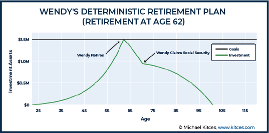
Example 1: Wendy is 22 years old and hopes to retire at age 62 with an intended account balance of $1.5 million. She has read about the benefits of delaying Social Security and plans to claim at 70 years old.
A straight-line analysis of her contributions (initially $300/month, rising by 3.5% per year) at a long-term expected return of 8% show that her plan is feasible.
The caveat to this example is that while returns may have averaged 8% on a long-term growth portfolio, in reality a wide range of potential outcomes may occur. The above fails to address the risk of potential shortfall that emerges once considering volatility and sequence of return risk.
Fixed-Decision Simulation Of Financial Planning Goals Can Show A Range Of Potential Results
Fixed-decision simulations provide a first step toward understanding a plan’s true risk (that isn’t sufficiently illustrated with a traditional straight-line-growth spreadsheet projection).
It allows the planner to input a set of client goals and shows the range of potential results around that goal, recognizing that markets don’t necessarily grow in a straight line (even if they tend to average out there over time).
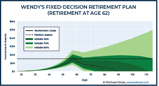
Example 2: After reviewing her straight-line analysis, Wendy requests another analysis that now shows the range of potential outcomes (assuming not just an 8% return on a growth portfolio, but a 12% standard deviation of returns around that average).
This analysis reveals that Wendy may in fact have a bit less or far more than her $1.5M target 40 years from now (by age 62).
Although her average retirement account balance at 62 is $1.5M, she falls short of her accumulation goal in about 50% of the simulations and runs out of savings as early as age 77 in about 15% of the trials.
As the chart above illustrates, it’s not enough to just recognize that there may be a range of results approaching age 62 depending on volatility. Because in practice, being far behind the retirement goal means that the client wouldn’t likely retire at that age in the first place!
In other words, it is usually impossible to decide a client’s retirement date early in the accumulation phase from Monte Carlo projections alone, because it’s not only wealth that is dynamic… but the retirement date itself, too!
Varying Retirement Dates Shows How Asset Accumulation, Social Security Benefits, and Retirement Funding Requirements Are Impacted
Clients can leverage the dynamic nature of their retirement age to reduce their risk of depleting their retirement portfolio. As while delaying retirement allows for more years of contributions and reduces the number of years in retirement that must be funded, it also adds extra years of work that can increase Social Security retirement benefit through a higher Average Indexed Monthly Earnings.
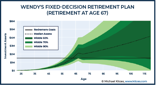
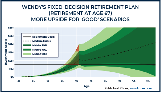
Example 3: To ameliorate her risk of an adverse outcome, Wendy adjusts her expectations. She requests another analysis that assumes she works until age 67 rather than age 62.
With the updated retirement age, she reaches her accumulation goal in about 85% of trials. While a risk of “failure” in retirement still remains, at least she has reduced her risk of “failure” (i.e., depleting the portfolio in retirement) to an-acceptable-to-her less than 5% by age 100 (i.e., a 95% probability of success).
By extending Wendy’s targeted age of retirement to reduce the frequency of failure, the potential upside increases, too, as Wendy’s adjusted plan allows even more time for the “good” scenarios to continue compounding upwards as well.
As a result, Wendy’s efforts to avoid failure are associated with a 15% probability of having more than $3M in wealth by age 67… far more than she needs to retire in the first place!
Given that the range of possible outcomes also includes trials in which the client’s returns are better than expected, retirement delays are not always necessary. Which may actually allow Wendy to enjoy a higher standard of living in retirement… or alternatively, to just retire earlier than the originally stated goal!
In fact, as the chart above highlights, although Wendy may have pushed out her planned retirement date from age 62 to age 67 to defend against the adverse outcomes, she also now has a 15% chance of reaching her original $1.5M goal as early as age 56 (just 34 years into her retirement accumulation plan). Which is important, because again in practice if returns are more (less) positive than expected, clients may want to retire sooner (later) than originally planned rather than accept a higher (lower) standard of living in retirement.
Or viewed another way, the “traditional” approach shows that Wendy can retire in 45 years at age 67, and at that age has a 15% probability of $3M or more in wealth (far above her original goal) alongside a 5% probability of failure by age 100.
A different way of framing the same plan is that Wendy has a 5% of running out of money after retiring at age 70 (if she lives to 100), and a 15% probability of having more than her asset goal by age 56!
To say the least, then, running simulations with fixed retirement dates may show the range of wealth around that particular retirement date… but does not actually provide a clear answer to the question “when can I retire?”!
Dynamic Retirement Dates and Sensible Asset Goals Can Be Modeled To Provide More Meaningful Outcomes
Working with dynamic retirement dates offers even more flexibility (and maybe even offering more realistic perspectives) to planning, as prospective retirees usually decide to retire when they actually feel they are ready. This date can be estimated, but not determined in advance, as it is often contingent on factors (such as investment returns) beyond individual control.
Simulation can help clients understand the range of potential retirement date outcomes associated with their plan, which may be more meaningful than asset values far off into the future. In this framework, investment assets are a means to an end, rather than an end to itself.
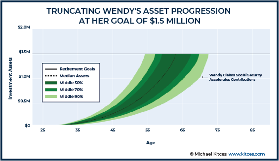
Truncating Wendy’s asset progression at her goal amount eliminates the noise created by the potential for ‘excess’ wealth that in practice Wendy wouldn’t accept (because she’d likely adapt the goal by retiring earlier instead of accumulating more beyond her needs). This adjusted chart can serve as a reference for clients as they track progress toward their retirement goal.
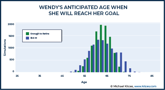
Example 5: Wendy’s simulation helps her understand how long it will take to acquire $1.5M of assets with her current contribution plan. On average, she obtains this goal in just over 40 years, but may achieve the goal in as few as 32 years, or as many as 50 years. Either way, she believes she will be prepared to retire when her goal is reached. Accordingly, the ‘excess’ wealth is truncated from the plot, because she plans to adjust her retirement date based on the path that unfolds.
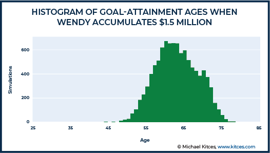
For those who don’t want to figure out exactly what ages the accumulation paths intersect with the goal line, an alternative approach is to create a histogram that simply illustrates the range of goal obtainment ages.
Yet while this appears to be a significant improvement, in showing the range of ages at which retirement can occur (instead of just the range of wealth shortfall or excess at a somewhat-arbitrarily-determined retirement goal date), it leaves an important question unanswered: when will she have enough to actually retire?
Flexible Retirement Wealth Goals Can Illustrate Flexible Retirement Date Options
The problem with projecting a range of retirement dates is that earlier dates of retirement will result in more years in retirement, while later dates of retirement have fewer years of retirement itself to support. Which is important, because it means that what Wendy needs to retire at age 50 is not the same as what she needs if she were to retire at age 75. In other words, the retirement savings need is not uniform across all of the retirement dates. Stated another way, making the retirement date more flexible is best implemented with a flexible retirement wealth goal as well – because different retirement dates have a different “goal cost”, too.
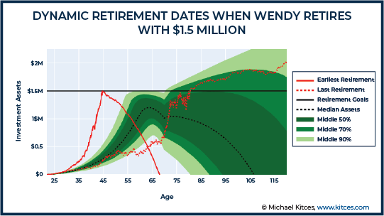
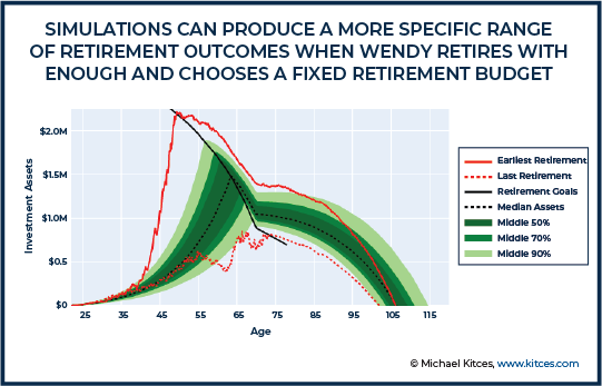
Example 6: Wendy’s advisor re-runs the simulation with a dynamic retirement date. The range of asset values is closer to her expectations, as she retires earlier when she accumulates wealth faster (rather than just accumulating more), and retires later if her path lags behind. However, this exercise still does not tell her when she will have enough.
The simulation path with the earliest accumulation goal achievement, represented by the solid red line, results in portfolio exhaustion by age 70. $1.5M is not enough for her to retire at age 45.
Equally troubling, she may still be short of her $1.5M goal at age 75. Not only would this delay likely be unacceptable to her, it is also unnecessary. The dotted red line, representing her latest goal achievement date, indicates a significant final estate, suggesting she did not need the full $1.5M and could have retired sooner.
This form of simulation is incomplete because it fails to incorporate the relationship between the retirement date and goal cost.
The Waring Siegel Rule in Reverse Can Model The Dynamic Relationship Between Target Goal Thresholds And Retirement Dates
If the cost of a goal in a client’s financial plan is fixed – e.g., a plan to retire upon achieving $1.5M of retirement assets – it’s just a matter of time until the goal line is crossed. The story becomes more complex, though, when the goal cost itself is dynamic as a result of the different time horizon in retirement (i.e., fewer or more years of retirement spending itself) that occurs when the time to the goal shifts sooner or later.
In this case, the visual goal line shift is determined by both the change in time to the goal, and the change in cost of the goal. A mental attribution becomes far more difficult, and difficult to communicate using asset-oriented reporting alone.
Annuities may be inappropriate for clients who have uneven spending desires, find the pricing unattractive, and/or have concern regarding the ability of the insurance company to make the payments. However, the price of an annuity can be a useful tool for estimating the assets required to support a client’s retirement budget.
In The Only Spending Rule Article You Will Ever Need, Waring and Siegel suggest those who prefer to self-insure longevity risk consider a withdrawal rate calculated using the average of an inflation adjusted (real) annuity for life expectancy and a real annuity for maximum life. This dynamic budgeting rule is designed to mitigate the risk of fully liquidating the portfolio and modestly front-loads spending to allow for more spending in the earlier years of retirement. The rule can be customized by shifting the weighting between maximum life and (average) life expectancy to match the client’s preferences.
Because this article is focused on the accumulation stage, the rule will be applied in the reverse direction. The chart below plots the assets required to impute an initial withdrawal rate of $1,000 (inflation indexed at 1.78% and age 70) per month using this rule, a maximum age of 120, the 2016 Social Security Period Life Table for a female, and return assumptions of 1.19% real and 2.97% nominal (the real yield of the 30 year TIP and the yield of the 30 year nominal treasury respectively as of the beginning of 2019).
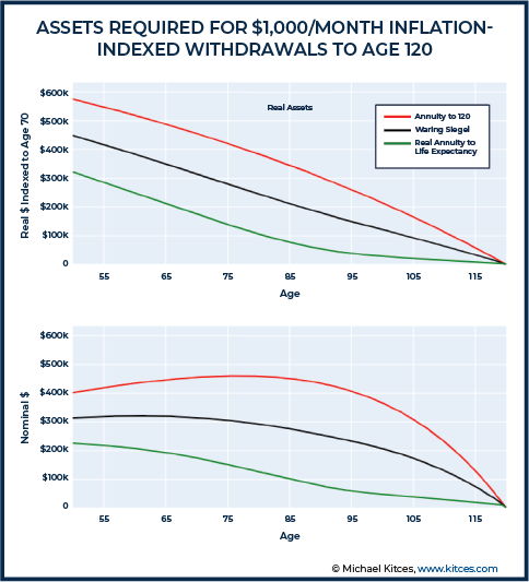
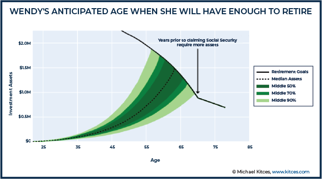
Notably, the end result of this chart is that the target goal threshold changes over time and exists on a diagonal, where the required assets (i.e., the goal cost) is higher in the earlier years and declines in the later years. It is not simply a horizontal goal line that truncates the ‘excess’ wealth once a fixed dollar amount goal is reached.
When applied in Wendy’s situation in particular, changing Wendy’s goal from “$1.5M of assets” to “an asset value sufficient to support, in combination with her Social Security benefit, $10,000/month expenditures growing at 1.78% (real) for life” appears to reduce her retirement date risk.
In this framework, the ‘best-case’ scenario actually takes longer (as she needs more if she retires early), but her worst-case scenario is shorter (as she won’t need as much if she retires later). This occurs because each year of delay reduces retirement life expectancy, reduces the number of years in retirement prior to receiving Social Security, and increases the Social Security benefit once received. All three reduce the size of the portfolio required to support her spending needs.
The charts below illustrate this narrowing of the range of outcomes by more accurately reflecting not just the dynamic retirement date but also the dynamic goal cost of that dynamic retirement date. And the retiree conversation is transformed from discussing a range of retirement wealth outcomes (and potential wealth shortfalls or excesses) into a range of potential retirement dates (i.e., years to retirement) instead.
Example 7: Wendy’s advisor uses the Waring Seigel Rule in reverse to estimate her assets required to impute an initial $10,000 per month budget.
As a result, her anticipated retirement age (from the 10th to 90th percentiles) falls between 58 and 68 years.
Although the Waring Seigel Rule is designed to ensure the client does not deplete their portfolio before some maximum age, some clients may prefer not to reduce spending as they age. Using it in reverse for the accumulation period can still be useful to model appropriate retirement dates, even if it is not expected to be used during retirement.
Example 8: Wendy decides to follow a fixed real budget rather than follow the Waring Seigel Rule in retirement.
Unlike the fixed asset goal simulation, which included paths resulting in early exhaustion and paths resulting in a sizable estate, this simulation produces a relatively narrow range of outcomes during the retirement phase.
In this simulation, she typically depletes her portfolio about halfway between her remaining life expectancy as of her retirement date and years remaining to 120. Depending on her longevity expectations, this may or may not be acceptable to her.
How Monte Carlo Simulation Techniques Can Be Used To Present Time-Centric Plans To Clients
People tend to focus on what is measured and readily observable. Asset values are easy for the client to monitor, even though they too often distract from the client’s goals, and therefore become a focus for prospective retirees monitoring their progress towards retirement (e.g, they may ask, “Is my wealth going up every year to get me closer to retirement?”).
In this context, time-centric reporting may help clients refocus on their goals (in addition to being better to project out those goals in the first place)… especially when contrasted with the future value of a coffee-a-day or other conveniences (a common trope in financial planning that fails to motivate clients to invest because the value and implications of the large sums of money far off into the future are difficult to internalize). However, further work is required to fully implement this time-centric shift in focus.
Tracking Assets and Time Over A Countdown-To-Retirement Graph Helps Clients Shift To A More Time-Centric Framework
When retirement liability is considered deterministic (i.e., when there is no allowance for random events to impact the analysis), it may be dynamic with respect to the retirement date but is nonetheless still non-random. It is ‘fixed’ with respect to the cost to fund the retirement goal (at whatever date that was triggered based on the goal’s dynamic cost). Unfortunately, the truth is far more complex.
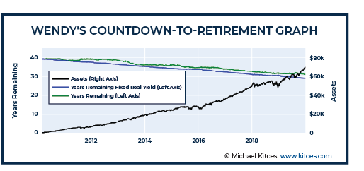
While account balances are generally readily available for clients in a number of locations, including account statements, custodian websites, and advisor web portals, another metric and illustration of progress is required to help accumulating clients shift to a time-centric framework. A countdown-to-retirement graph could serve this purpose.
For example, in 2019, the 30-year real interest rate fell from 1.19% to 0.58%. Using the Waring Seigel Rule, the assets required for a 66-year-old to retire increased by about 13% (because of the high implied cost embedded in lower future return assumptions)! In early years, changes in the projected future cost of retirement may be larger than the investor’s entire account balance. Adding further insult to injury, expected returns should arguably be adjusted downward in the future in general, at least for fixed income.
By regularly re-pricing the investor’s goal, advisors can help young clients recognize that the biggest risk to their retirement plan is often not the stock market. And the closer they are to the retirement goal, the shorter the countdown of their years to retirement (even as the goal itself changes over time).
This is an important contrast to just tracking wealth towards retirement, which in real dollar terms becomes more volatile as retirement approaches (and there’s literally a larger portfolio on which market volatility compounds).
Example 9: Despite being 100% invested in global stocks during a 10-year bull market (and generating an annual internal rate of return of 10%), Wendy’s expected time to retirement has only fallen about 9 years as the decline in the 30-year real interest rate from 2.22% on February 22, 2010 to 0.58% at the end of 2019 caused her retirement goal cost to keep pace with her rapid accumulation of retirement assets.
If the interest rate had remained the same (blue line), she would have been about 1 year ahead of schedule rather than 1 year behind (green line).
Increasing Goal Costs Can Be Illustrated To Help Clients Adjust Saving And Spending Patterns
Although adding a single line representing the expected liability progression can help clients begin thinking in a liability-driven investing framework, the asset cone graph does not easily integrate the progression of what may be an uncertain liability itself. Fortunately, a histogram is still applicable and can help to illustrate the point.
Example 10: Henry is a recent graduate who lives with his parents. This allows him to maximize his savings toward his goal of purchasing his first home, a condo in San Francisco.
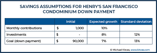
He estimates the current cost of the home he desires is about $0.9M and would like to use a 10% down payment.
His advisor, using annual condo appreciation data from FRED (that shows the goal – the condo itself – will also get more expensive as home values grow while Henry is saving), makes the following assumptions:
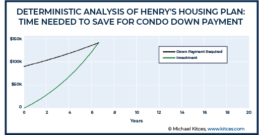
A deterministic analysis suggests it will take Henry about 7 years to save for his down-payment.
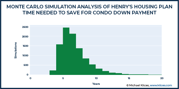
Using Monte Carlo simulation tools, an initial analysis shows it will take between 4.5 and 9.5 years at the 10th and 90th percentiles.
When the goal cost is expected to increase, worst-case scenarios can result in significant delays. A higher contribution rate can help reduce both the expected time and the delay risk by reducing the amount of time the liability has to grow.
Time-Centric Reporting Facilitates Sensitivity Analysis
Over many years, implementing or changing small habits can have a large cumulative impact. Advisors can illustrate the impact of these small changes by measuring outcomes in terms of time, which can also make the impact more relatable to the client.
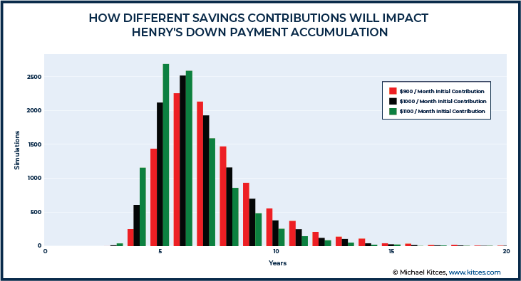
Example 11: Henry asks if changing his contribution rate would reduce his potential wait to move into his new home.
His advisor re-runs the simulation using a 0.25 correlation between the home price and the investments (since faster growth in home prices also tends to be correlated to faster growth in markets overall and the positive wealth effect that occurs), and shows that a $100 per month increase to his initial contribution rate could reduce his probability of waiting 10 or more years to less than 5%, but a decrease would increase his probability of an extended wait to more than 10%.
A $100 per month change in his contribution rate would change his expected wait time by about 200 days on average.
Transitioning clients from an asset framework to a liability-driven investing perspective is an uphill climb, not only because of the complexity, but also because of the low interest rate environment (as low discount rates are especially sensitive to changes in the implied cost of time-related goals).
Nonetheless, the concept of time is easier for most clients to understand than funded status, and by incorporating time-based factors into financial planning software used to project and track financial planning goals, advisors can leverage sophisticated financial planning techniques without confusing their clients about the impact of financial trade-offs and keeping those clients focused on how they are progressing towards their goals over time.




Hasn’t this sort of thing been an ongoing theme in Larry Frank’s work?
How would an average planner be able to show a client these things given the tools and knowledge they likely have: Excel and a financial planning software
very detailed article.Retirement planning is the process of figuring out how much money you’ll need to save for retirement and then putting a plan in place to get there. Retirement isn’t an age—it’s a financial number! Be confident about your retirement.