
Executive Summary
For most people, making financial planning decisions involves an evaluation of financial trade-offs. In fact, any decision about whether to save (or not) effectively boils down to a trade-off about whether to consume now, or later.
Of course, all else being equal, we virtually always choose to consume now, if we can. Delaying gratification requires at least some kind of incentive, to make it worth delaying. Or viewed another way, we “discount” the value of something in the future – because we have to wait for it – which means waiting must make something more valuable to ever be worth the wait.
Mathematically, we can quantify this “time value of money” as a discount rate, which represents the rate of growth that would have to be earned to make the waiting worthwhile. And the use of a discount rate is especially helpful when trying to compare strategies or choices that are dispersed or occur over time, where it’s not always intuitively obvious which is the better deal in the long run.
For instance, discount rates are used to evaluate whether it’s better to take a lump sum rather than ongoing pension payments, and to determine when it’s preferable to wait for (higher) Social Security payments, rather than starting early… both of which are trade-offs that entail payments over a span of years or even decades, and can be difficult to compare without a common framework. By calculating the "net present value" of the various alternatives, adjusted by an appropriate discount rate of interest, it's feasible to make better apples-to-apples comparisons.
The caveat, however, is that conducting such analyses still requires an appropriate choice for a discount rate of interest in the first place. In the context of financial planning strategies, the proper discount rate to use is literally the “time value of the money” for that individual – in other words, what return could be generated over time by the money, if it were in fact available today to be invested. Or stated more simply: the discount rate for financial planning strategies should be the long-term rate of return being assumed in the financial plan itself. Because it’s the portfolio to which the money could be added if taken earlier, and/or it’s the portfolio that will have to be liquidated to provide for spending needs if the payments are delayed until later.
Notably, the fact that the proper discount rate is the investor’s expected rate of return, means that the “right” discount rate will vary from one person to the next, based on their investment approach and risk tolerance. For those who are more inclined towards aggressive investments, a higher discount rate may be used, while those who are conservative will use a lower discount rate of interest (and those who hold all assets in cash might well use a discount rate near 0%!). Of course, the caveat is that investors must still be cautious to pick a discount rate that is actually realistic to the portfolio in the first place – otherwise, an unrealistically high discount rate will lead to decisions that turn out to be less-than-optimal after the fact, when the money-in-hand doesn’t actually produce the expected results!

The Discount Rate And The Time Value Of Money
Evaluating any trade-off involves weighing the pros and cons of choice “A” versus choice “B”.
When the outcome of the choices is also immediate, the comparison is relatively straightforward. If I’m trying to decide whether to spend $1,000 to take a vacation, I can weigh the perceived benefits of the vacation (fun, enjoyment, relaxation, a chance to see a new part of the world) against the cost ($1,000 that I won’t have anymore), and make a decision.
However, the choice is inherently more complex when the trade-off entails outcomes that occur at different points in time. For instance, if I’m trying to decide whether to take a vacation this year, or to take one next year instead. Naturally, given a desire for (instant) gratification, there’s little incentive to wait to take a vacation, if an equivalent one is available immediately; instead, waiting is only appealing if there’s some benefit to doing so. In other words, we demand that if we’re going to wait, the value must be somehow enhanced by waiting (i.e., a better vacation a year from now than the one I could simply take today). Or viewed another way, we “discount” the value of a vacation occurring in a year compared to a vacation we can take now, which means for an otherwise-equivalent vacation, it’s more valuable to take the immediate (undiscounted) choice.
Mathematically, this discounting-the-future effect means that we can calculate a “discount rate”, which represents the breakeven rate of return that would have to be generated between now and then to compensate for the waiting period. For instance, if the discount rate was 5%, it means that I would only be willing to wait on the vacation for a year, if the vacation I got to take in a year was 5% “better” (e.g., by growing my money by 5% so I have that much more to spend on the vacation).
Of course, when it comes to something as personal and intangible as a vacation, it can be difficult to quantify an exact discount rate. And there’s some research to suggest that we are not always rational in applying discount rates to personal trade-offs over time – and that we tend to engage in “hyperbolic” discounting of the future.
On the other hand, when evaluating an investment decision or trade-off, we can much more effectively evaluate the trade-off by recognizing that future investment outcomes (or future cash flows) need to be discounted if there’s a waiting period, to recognize the implicit “time value of money”. Which means the discount rate quickly becomes an essential component to weighing investment and financial trade-offs over time.
Discounted Cash Flow (DCF) Valuations Of A Stock (Or Advisory Firm)
One of the most common applications of using a discount rate to evaluate an investment decision is the use of the Discounted Cash Flow (DCF) model to evaluate whether it’s worthwhile to buy a company’s stock (or not).
The essence of the analysis is relatively straightforward: estimate every cash flow that the business is likely to provide in the future (some combination of its ongoing dividend/profit distributions, and its terminal value for payments in perpetuity as a stable business thereafter), and then discount the value of those future cash flows back into today’s dollars. If the discounted “present value” of the future cash flows is higher than the actual price to buy the company, then it’s a good buying opportunity (because the actual price is cheaper than the intrinsic present-value-of-future-cash-flows price). If the stock costs more than the present value of its future cash flows, it’s overpriced and the investor should pass.
The caveat, however, is that estimating the discounted present value of future cash flows has two key assumptions: the first is what those future cash flows will actually be, and the second is the discount rate itself. And while determining the future cash flows of a business is beyond the scope of this discussion, the key point is that a prospective investment could be a good deal, or a bad one, depending on the discount rate alone.
Example 1. Jeremy is considering whether to buy a company for $1,000,000. Over the next 5 years, it is estimated to generate $40,000/year of profit distributions, and by the end of the time period, is projected to be worth $1.1M. Which means the cash flows are $40,000/year for the next 4 years, with a total final payment of $1,140,000 at the end of the 5th year (which represents the last profit distribution, plus the $1.1M terminal value).
At a 5% discount rate, the present value of these future cash flows is $1,035,058, which makes the stock an appealing investment at “just” a $1,000,000 price. On the other hand, if Jeremy had an opportunity to invest into another company that had a 10% expected return – such that he required at least a 10% discount rate to invest in this company as a superior alternative – the outcome would be different. Using a 10% discount rate, the company is only worth $834,645, which means buying it for $1,000,000 would be a “bad” deal that overpays for its value – even though cumulatively, Jeremy would receive back $1.3M in total payments over the next 5 years, that’s actually less than what Jeremy could have generated by simply keeping his $1,000,000 and invested it at his 10% 'required' rate of return over that time period.
Notably, the key determinant of the discount rate is not based on the investment itself, per se, but on the opportunity cost of using that money in lieu of some other alternative, instead. For instance, in the example above, Jeremy’s decision to use a 10% discount rate was based on having a (comparable risk) alternative investment that already had an expected return of 10%, which effectively became the “hurdle rate” that the new investment had to clear (and in this case, couldn’t surpass). In the business context, projects are often evaluating using a discount rate of the Weighted Average Cost of Capital (WACC), in recognition that if the prospective returns on the investment of capital can’t surpass the cost of the capital, then the cost will exceed the outcome, which again would make it a losing proposition.
Determining An Appropriate Discount Rate Of Interest For Financial Planning Strategies
While it may seem an abstract exercise, in reality determining an appropriate “discount rate” is actually highly relevant when evaluating many financial planning strategies, particularly ones that compare traditional investment opportunities with fixed cash flows over time, such as whether to take a lump sum pension (or not), or the value of delaying Social Security benefits (or not).
In both scenarios, the discount rate effectively forms a “hurdle rate” of expected value that the strategy must surpass to be viable/desirable (and if the discount rate can’t be exceeded, the strategy shouldn’t be implemented).
Pension Vs Lump Sum Discount Rate
A pension is a guaranteed lifetime stream of cash flows, which inherently makes it difficult to evaluate relative to other more traditional investment alternatives. Of course, as long as someone has only a pension available to them, there’s no decision to make, and the payments will simply be made. However, once there’s an option to take the pension or convert it to a lump sum, the question arises: How do you determine when/whether the lump sum is a “good deal” or not? To which the answer is: Calculate the present value of the pension at an appropriate discount rate, and see if it’s more or less than the lump sum amount being made available.
Example 2. Charlie is a 65-year-old male, and is eligible for a $40,000/year lifetime pension. The company has also offered Charlie a $500,000 lump sum option, in exchange for his pension, and he’s trying to decide if this is a “good” deal or not. According to the Society of Actuaries’ Longevity Illustrator, as a non-smoking male with reasonable health, Charlie’s life expectancy is approximately age 87, which means he can expect to receive $40,000/year for an average of 22 years.
Charlie’s alternative, if he takes the lump sum, would be investing it in a diversified portfolio, in which he estimates that he could earn a 7% average annual growth rate. Which means that potential portfolio return is the opportunity cost he’s giving up if he sticks with the pension and doesn’t take the lump sum. Thus, 7% would be Charlie’s discount rate.
If Charlie then calculates the present value of his $40,000 year for 22 years at a 7% discount rate, he’ll find that the net present value is “only” about $451,000. In other words, it would only take $451,000 to provide $40,000/year for 22 years at a 7% rate of return. Since the available lump sum provides more than that – a full $500,000 – this implies that it’s a slightly better deal to take the lump sum, since it would literally give Charlie “more than enough” to replace his 22 years of pension payments at a 7% rate of return (with almost $50,000 to spare!).
Another way of evaluating the decision of whether to take a pension lump sum or not is to calculate what discount rate is actually being used to provide the pension lump sum. After all, mathematically, if there’s a stream of pension payments already available, and a lump sum being offered as a choice, there is some discount rate that will equate the projected pension payments to the lump sum being offered. This internal rate of return on the pension lump sum itself provides the “hurdle rate” that the lump sum would have to achieve, if subsequently invested, to actually replicate the exact pension payments (to the dollar, with none left over).
Example 2b. Continuing the prior example, if Charlie’s trade-off is a $500,000 lump sum, or to receive $40,000/year for the next 22 years, we can calculate the internal rate of return (IRR) of this trade-off (the discount rate that would make the two precisely equal to each other).
In this case, the IRR would be 5.8%, which means that $500,000 growing at 5.8%/year while withdrawing $40,000/year would last for exactly 22 years (with nothing left over). To the extent that the lump sum investor could earn anything greater than 5.8%, there would be money left over; thus, as long as Charlie is confident he can earn at least 5.8% (and that 22 years is a reasonable time horizon), it’s a better deal to take the lump sum to cover his needs for the next 22 years, and invest it accordingly. (In turn, this is why it was a "good" deal to take the $500,000 if Charlie's discount rate was 7% - because his 7% assumed return is enough to beat the 5.8% hurdle rate.)
Notably, an important caveat to applying a discount rate for valuing a pension is that it’s still necessary to determine the cash flows to discount in the first place – in other words, what are the pension payments, and how many years of expected pension payments there will be. Of course, this is ultimately an unknown, particularly for an individual; while on average 65-year-old males like Charlie may leave to age 87 (which can be predicted fairly accurately thanks to the law of large numbers), Charlie himself might live much longer or shorter than this time period. Which matters because having a longer time period, and receiving more pension payments, improves the internal rate of return of the pension compared to the lump sum, and makes the pension inherently more valuable.
As a result, effectively evaluating the discount rate on a pension-vs-lump-sum decision really requires calculating the implied value over multiple different time horizons, to understand not only whether the lump sum is a “good deal” or not at the available discount rate, but also the risk that the outcome/decision would be different if the pensioner lives longer or shorter than the mere average life expectancy.
Accordingly, the chart below shows the internal rate of return for Charlie, and how it changes as each additional pension payment is received from age 65 all the way to age 100. Not surprisingly, early on the internal rate of return of the pension is hugely negative – a tremendous loss to take “lifetime” payments and pass away after getting just a few – but if Charlie lives long enough, eventually the internal rate of return turns positive at age 76, climbs to 3% by the time he’s 80%, over 6% by the time he’s 90, and goes all the way to 7.4% by age 100! Alternatively, this means that if Charlie calculates the present value of the pension payments at his 7% discount rate, its value will be less than the pension lump sum (implying the lump sum is a “good deal” to take)… until/unless Charlie lives into his late 90s, and then suddenly the pension itself turns out to be the better deal after all!
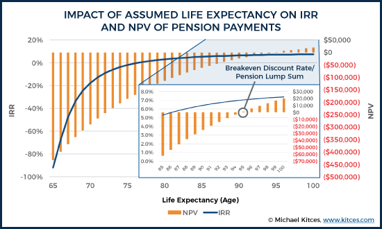
In all cases, though, the fundamental point of the discount rate remains the same: it represents the opportunity cost of not taking the lump sum and investing it (and spending from it), and should be compared to the available investment rate of return in the portfolio. The higher the expected rate of return – the better the investment opportunities for the lump sum – the more discounted (i.e., reduced in value) the guaranteed pension payments will be, and the more appealing it will be to simply take and invest the lump sum. Alternatively, the lower and more conservative the expected rate of return (and thus the discount rate), the more valuable (and literally, the “less discounted”) the guaranteed pension payments will be!
Discount Rate For Delayed Social Security
The decision of whether to delay Social Security benefits to age 70, or not, represents another kind of “discount rate” analysis. In this case, the challenge is that both alternatives – take lifetime payments early, or wait and take higher lifetime payments starting later – involve a series of lifetime payments over the span of years and decades, but with different starting points, which makes them difficult to compare.
As a result, one of the most common approaches to evaluating Social Security trade-offs is to calculate the discounted net present value (NPV) of each choice, and then see which one has the higher value. Converting each to a discounted present value allows them to be compared on equal footing.
Here again, though, the choice of a discount rate is both necessary, and critical to the analysis. The reason the discount rate matters is that its value – and the magnitude of (compounded) discounting it applies to distant future payments – can directly tilt the scales for or against strategies that give larger future payments over smaller current ones.
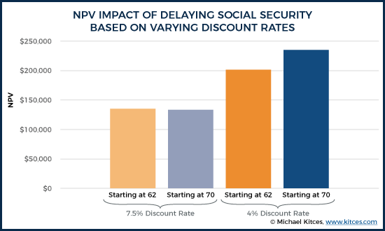
Example 3. Ashley is a 62-year-old female, trying to decide whether to start Social Security benefits early (now, at age 62), or delay them until age 70. Her Primary Insurance Amount (PIA, or the benefit she’ll receive at full retirement age of 66) is $1,000/month. If she starts at benefits now, her payments will be reduced by 25% to $750/month. If she waits until age 70, the payments will be increased by 32% for delayed retirement credits, all the way up to $1,320/month (plus additional cost-of-living adjustments between now and then). The fundamental question: which is more valuable, $750/month starting today, or $1,320/month starting 8 years from now?
Assuming Ashley will live to age 88 (based on the Society of Actuaries’ Longevity Illustrator for a 62-year-old female non-smoker with average health), and assuming 3%/year cost-of-living adjustments for inflation and a 7.5% discount rate, the present value of taking payments early is $135,204, while delaying them would have a value of $133,496, which tilts the scales slightly in favor of just taking the payments early, and investing them for that 7.5%/year potential return.
On the other hand, if Ashley's opportunity cost of the money is only 4%/year – perhaps as an investor she is far more conservative – then the higher future payments are more valuable (literally, less discounted), and now the present value of starting early is only $201,764, while the value of starting at age 70 is $235,477, which tilts the scales towards delaying.
As the example here shows, the choice of the discount rate is once again crucial to the outcome of the decision. Which once again raises the question of what discount rate should be used?
Given that a discount rate represents the implicit “time value” of the dollars, and the opportunity cost of the money if it is not received until later, the discount rate should represent whatever could/would have been done with those dollars in the meantime. In other words, had Ashley not delayed Social Security, and taken the payments early instead, what would have happened to the money?
Assuming Ashley had a choice in the first place (i.e., she didn’t “need” the money as her sole source of spending, and had other resources available), choosing to take Social Security benefits early represents either an opportunity for Ashley to invest the payments into her portfolio, or alternatively meant she could have spent those payments and not had to withdraw from her portfolio instead. Either way, the opportunity cost of delaying is the dollars for the portfolio that are not saved, or the dollars from the portfolio that would have to be withdrawn/liquidated/spent while waiting for Social Security. Which means the portfolio’s expected rate of return is, once again, the appropriate discount rate.
Notably, this will provide the same decision outcome as simply projecting Ashley’s retirement planning situation, using a combination of her available retirement assets, and the Social Security payments, at the portfolio's assumed rate of return in the financial plan.
Example 3b. Continuing the prior example, assume that Ashley’s overall goal is to spend $35,000/year, and that in addition to her Social Security payments, she also has a $500,000 portfolio. In this scenario, she will either begin to draw immediately on Social Security and supplement her spending with her portfolio, or she will draw more heavily from her portfolio early on and then much less once Social Security begins (at the higher amount) at age 70. The chart below shows the outcomes of the two scenarios, assuming either a 4% portfolio return or a 7.5% portfolio return.
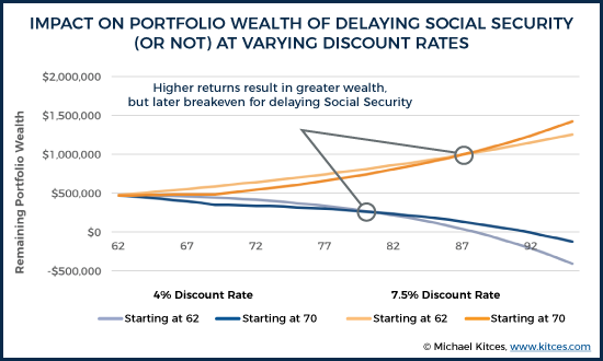
Notably, the conclusion is exactly the same as shown earlier – the higher the portfolio return, the less value there is to delaying (i.e., the longer the breakeven period to recover the 'cost' of waiting), and the more beneficial it is to simply start Social Security early, preserving more of the portfolio to stay invested at that 7% return; conversely, when returns are lower, the increase in Social Security payments by delaying is relatively more appealing. In fact, this is the whole point of why the proper discount rate is the portfolio’s assumed rate of return – because that’s precisely what those dollars are projected to earn (either directly or indirectly) if payments start early.
Portfolio Returns And The Opportunity Cost Of Money
Ultimately, the key point is that evaluating strategies that involve trade-offs over time requires the use of a discount rate, and for the typical investor, the discount rate should be the expected return of the portfolio, which literally reflects the opportunity cost of the money for that individual (i.e., how the funds could be deployed if they were received sooner, rather than later).
Notably, this means that investors who are more aggressive and have higher expected returns will use a higher discount rate, which will naturally “bias” trade-offs towards getting money sooner rather than later – i.e., taking the lump sum in lieu of lifetime pension payments, or starting Social Security early instead of delaying it. Logically, this makes sense: for investors who are that optimistic about their ability to grow their assets, the best strategy is to get those dollars in hand as quickly as possible, and invest them (or at least, use them so other portfolio assets can stay invested and don’t have to be liquidated).
Conversely, those who are invested more conservatively – including those who don’t invest at all – will utilize potentially much lower discount rates, which inherently makes “delayed dollars” strategies more appealing (literally, “less discounted”). After all, if the money was just going to sit in cash or CDs anyway, there’s not much growth potential to having those dollars in hand, and it’s more appealing to just get higher payments later instead (even if they’re only “slightly” higher).
It’s important to note, though, that despite the fact that Social Security and pension payments are themselves “fixed income” streams, their discount rate in a financial planning analysis is not necessarily using a fixed income return, unless the individual would truly have put all of those dollars into fixed income investments if the money was available now (e.g., as a pension lump sum, or by starting Social Security early). It is true that the payment streams themselves are fixed, but evaluating the trade-off means not calculating the fixed-income “value” of Social Security or a pension, per se, but its value as a trade-off to available alternatives (that the portfolio would have otherwise funded). By analogy, if you were considering whether to liquidate a bond to purchase a stock, the fundamental question is the earning potential of the stock, not the value of the bond itself as a fixed-income investment. Similarly, the decision about whether to start Social Security early, or take a pension lump sum, is not about the fact that it’s a fixed-income payment, but the (portfolio’s) opportunity cost and potential return it can generate by getting those fixed payments in hand sooner rather than later.
Alternatively, it’s also feasible to evaluate such trade-offs by calculating the internal rate of return of the cash flows themselves – whether it’s “giving up” current Social Security payments to receive higher payments later, or giving up a lump sum now to receive pension payments for life. The internal rate of return of those cash flows reveals the implicit “hurdle rate” that an alternative strategy – e.g., an investment portfolio – would have to beat to achieve a superior outcome. (Recognizing that the IRR itself will vary depending on the time horizon chosen, at least for pension and Social Security payments that continue “for life”.)
Of course, it’s still important to choose a realistic rate of return for the portfolio as a discount rate – or risk that a strategy “looks” appealing based on a too-high discount rate, and turns out to be a bad decision because that return isn’t actually achieved. Analyzing retirement planning trade-offs using tools like Monte Carlo analysis can at least help to identify these potential issues, as Monte Carlo inherently recognizes a range of possible returns, and can spot scenarios where a strategy may only be marginally superior – for instance, there’s a big difference between a pension lump sum that has a 95% probability of being superior, versus just a 51% chance, even if both are an “odds-on” bet with a favorable discounted net present value. And more generally, conservative investors should choose more conservative discount rates, while aggressive investors select more aggressive discount rates, simply to reflect how the available dollars really would/could be invested. Those who truly hold assets in cash might well use a discount rate near zero, to reflect that (current) reality.
The bottom line, though, is simply to recognize that using a discount rate can be a very effective means of evaluating the relative value of different strategies that provide varying payments over time, and comparing strategies to each other. But when analyzing those situations, it’s crucial to use a discount rate that appropriately reflects the opportunity cost of those dollars to the individual situation (whether it’s money to invest, or otherwise preserves portfolio dollars from not being withdrawn or liquidated so that they can remain invested).
So what do you think? What do you assume as the discount rate when doing a pension or Social Security analysis? Is it different for a pension lump sum decision? How do you explain your discount rate assumption? Please share your thoughts in the comments below!
