Executive Summary
The sustainability of retirement cash flows from a portfolio depends in no small part on the returns generated by that portfolio – in particular, the real returns, given the pernicious impact of inflation over a multi-decade retirement.
In today’s high-valuation environment, many retirement projections are being done with reduced long-term return assumptions… with the caveat that while many advisors agree on the need to project lower returns, there is little agreement on how much lower it should be.
A look at the available market data suggests that realistically, it would be appropriate to reduce equity return assumptions by about 100bps (or 1 percentage point) over the next 30 years, to reflect the current valuation environment. Ironically, the reduction is not greater, because 30 years is such a long time that even if returns are bad for a period of time, there are enough subsequent years to recover as well.
In point of fact, though, it turns out that market valuation is even more predictive of 15-year returns, and that today’s high P/E ratios imply that between now and 2030, market returns could be reduced by as much as 400bps. On the other hand, because market valuations (and the associated returns) tend to move in cycles, this also implies that in the 2030s and 2040s, market returns could be as much as 400bps above the long-term average as well.
Ultimately, then, the ideal way to adjust return assumptions in a retirement plan in today’s environment may not be to reduce long-term returns at all, but instead to do projections with a “regime-based” approach to return assumptions. This would entail projecting a period of much lower returns, followed by a subsequent period of higher returns, in a manner that more accurately reflects the impact of market valuation on returns – and better accounts for the sequence-of-return risk along the way as well!
Impact Of Market Valuation On Long-Term Equity Returns
As Benjamin Graham famously said, “in the short run, the market is a voting machine but in the long run, it is a weighing machine.” The fundamental point that the father of value investing was trying to make: while in the short term market prices generally move based on the market psychology of what’s popular (and not necessarily based on what the investment is “really” worth), in the long run markets eventually weigh an investment based on its underlying value.
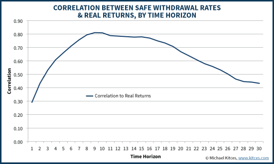
And as the data reveals, this phenomenon really is true; in the short run, market returns exhibit little relationship with their underlying market valuation (the correlation between returns and valuation is low). Over longer term time periods, though, market valuation actually exhibits a remarkably high correlation with subsequent compounded market returns! For instance, the chart below shows the correlation between the overall P/E levels of the market (based on the Shiller CAPE) and subsequent returns of various time periods. The longer the time horizon, the better the correlation between market valuation and the returns that follow.
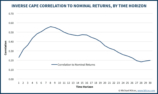
On the other hand, the data also reveals that in the ultra long term (e.g., 20+ years), market valuation actually becomes less predictive of equity returns. In other words, while market valuation is predictive for long(er) term market returns, eventually so much time has passed – and so much has changed – that the starting valuation is just no longer predictive of how markets grow and compound 20-30 years later. In fact, valuation is even less predictive of 30-year returns than it is in predicting 12-month returns!
Shiller CAPE And Real Equity Returns
Of course, the caveat to the chart above is that in the end, it’s not just about nominal investment returns to fuel long-term retirement spending, but real investment returns. After all, if the whole point of having equities for growth in the portfolio is to allow the portfolio to maintain spending power, it’s necessary for the equities to actually generate a favorable real rate of return.
Ironically, though, as it turns out, market valuation measures like Shiller CAPE are actually even more predictive of real market returns than it is just nominal returns! Or viewed another way, one of the reasons why long-term nominal returns are not well predicted by market valuation alone is that inflation confounds the picture. Yet since the ultimate goal is to project based on real returns anyway, using market valuation to predict real returns is just even more predictive!
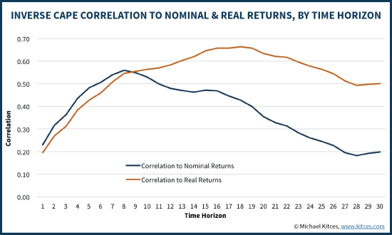
As the chart reveals, there is a correlation of almost 0.50 between the Shiller P/E ratio at the beginning of a time period, and the 30-year average annual real compound return that follows from the initial market valuation starting point.
In addition, the data reveals that the predictive relationship holds up in both higher valuation environments, and lower ones. For instance, the chart below shows the 30-year average annual compound growth rates for every starting year going back to 1871; time periods with starting valuations in the top 20% (a Shiller CAPE above 22) are colored red, while those with starting valuations in the bottom 20% (Shiller CAPE below 12) are green, and the rest (somewhere in the “muddled middle” 60%) are blue. Overall, the average 30-year real return is 6.3%, but while there is some variance of returns from high and low starting valuations, overall as expected the average of the high valuation zones is only 5.5%, while the lower valuation zones produced a 7.5% average return.
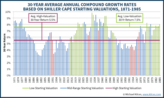
Notably, these results also suggest that even at valuation extremes, it would not be appropriate to adjust long-term equity returns by more than about 1% (or 100bps) in either direction. Which means even in today’s high valuation environment, where the Shiller CAPE is about 25.9, at the most it would only be appropriate to reduce long-term returns by 100bps.
30-Year Returns Are Comprised Of 15-Year Secular Bull and Bear Market Cycles
One important caveat to using market valuation to project 30-year return expectations is that, as noted earlier, while there is a significant correlation between Shiller CAPE and subsequent market returns, the peak correlation is actually after the first 15 years, and falls thereafter.
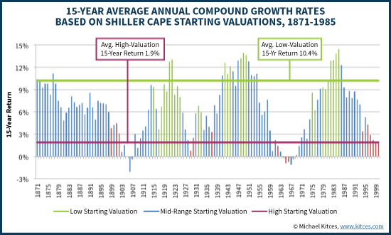
Over that first 15-year period, though, valuation is even more predictive of returns. For instance, the chart below shows the rolling 15-year real returns on equities, again segmented by whether the starting valuation was high, low, or in the middle. While over 30 years, market valuation suggests that the long-term return should only be changed about 100bps above or below the overall average, on a 15-year basis low-valuation environments have an average real return of 10.4% while high-valuation environments average only 1.9%!
On the other hand, while market valuation is more predictive of the first 15-year period than the whole 30-year period, it turns out that the subsequent 15 years aren’t entirely “random” either. In fact, because markets tend to move in cycles, especially poor 15-year returns in one period end out being predictive of good 15-year returns in the subsequent period.
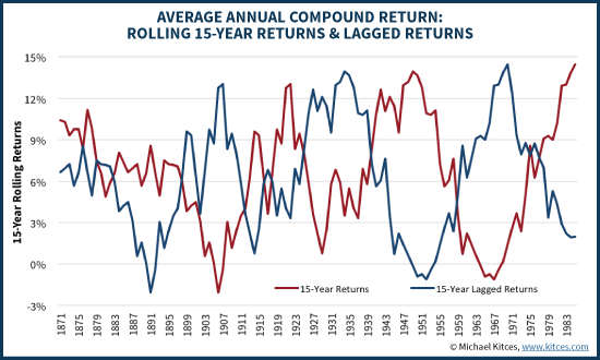
The chart above shows, for any given starting year, the average annual compound return in the first 15 years (red line), and the average annual compound return for the second (subsequent) 15 years (blue line). For instance, the first data point in red is, starting in 1871, the 15-year average annual compound equity return from 1871 to 1885 (15 years inclusive), while the blue line is the subsequent 15-year return from 1886 to 1900 (or the 15-year-lagged 15-year returns).
What the chart reveals is that bad 15-year returns in the market tend to be followed by good 15-year returns. The lines move in nearly perfect opposition to each other. Thus, there’s actually a 0.67 correlation between market valuation and subsequent 15 year returns, but there’s also an inverse -0.32 correlation between market valuation and the 15-year-lagged 15-year returns that follow!
In other words, high valuation actually predicts good future returns beginning in 15+ years, albeit only at a “cost” of bad 15-year returns between now and then. In today’s context of high market valuation, this implies below-average returns between now and 2030, but unusually high above-average returns in the 2030s and 2040s!
Regime-Based Equity Return Expectations For Retirement Projections
The key point of cyclical market returns is that just looking at market valuation to adjust (or in today’s environment, reduce) long-term returns actually misses out on an even more meaningful relationship between starting market valuation and alternating 15-year cycles that tend to follow. While market valuation extremes indicate 30-year returns may deviate by +/- 100bps, the valuation extremes indicate that 15-year returns may deviate by a whopping +/- 400bps (and tend to alternative)!
And the fact that market valuation predicts 15-year market cycles so effectively is especially important given that, for retirees, the sequence of returns early in retirement has a significant impact on the long-term sustainability of the retirement withdrawals. After all, the safe withdrawal rate is actually far more correlated to 15-year real returns that it is to 30-year real returns!
The significance of this dynamic is that it actually illustrates a significant “gap” in today’s retirement planning software. What the data suggests in a high-valuation environment today is that a “good” solution would be to reduce the long-term equity return by 100bps, but a “better” solution would be to illustrate 15 years of significantly below average real returns (e.g. reduced by 400bps), followed by 15 years of significantly above average real returns (increased by 400bps above the average!).
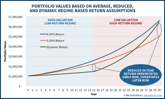
In other words, the optimal way to adjust retirement projections for extreme levels of high market valuation is not to reduce long-term returns by a little, but to reduce “intermediate” term returns by a lot for the current low-return “regime”, followed by a subsequent period of significantly higher returns (as the first 15 years of low returns amidst any level of ongoing economic growth eventually results in a low return environment). Doing so is superior because it more properly matches the true risk of high-valuation environments: exacerbated exposure to sequence of return risk, as valuation extremes trigger an especially high likelihood of a bad decade of returns, which is especially problematic for retirees sensitive to the first decade’s worth of returns!
Sadly, though, today’s financial planning software packages are incapable of modeling regime-based retirement projections – not because it’s impossible, or even difficult, to program, but simply because it’s not be programmed to do so. Hopefully that will change soon!
So what do you think? What equity return assumptions are you using for retirement projections? Are you reducing returns in today's environment? If so, by how much? Please share in the comments below!
Ravi says
Makes a lot of sense. However, while US CAPE is elevated, it is much less so internationally, and approaching the historical average for EM (shorter data series). Given the relative attractiveness of Non-US, it would make sense to have a portfolio of stable assets for 10 years worth of cash flow married with disproportionately Non-US holdings. With regards to planning software, I’d imagine you could add a cash outflow to mimic a lower return environment for as long as needed. While high valuations have good predictive measure of lower returns, they also come with a higher probability of greater draw downs. That would also have to be incorporated into the retirement projection.
Bill Cason says
Michael,
Great article and much appropriate to my personal situation as I have just retired. I follow your work closely as it provides a great amount of excellent info that I factor into our planning.
Regarding lack of modeling software, it does occur to me that I can “simulate” changes in portfolio performance (low for next 15 years; then high for the balance of our expected lives) using ESPlanner as I can forecast changes in portfolio content (cash, stocks, bonds, etc) for each year going forward. For example i could forecast being cash heavy in the near term and “simulate” poor returns.
Any thoughts on this?
Once again much thx for the great work you publish.
Bill
Kris Johnson says
Naviplan has actually had this capability for several years, though I believe it is done at the account level rather than globally. We actually switched away from Naviplan for other reasons, but just a point that at least one fairly well known planning software allows for this.
Hi Kris,
I use Naviplan. I am able to set separate returns for “pre-retirement” and “retirement” years, but I’m not aware of any way to establish different returns based on particular times horizons, such as “years 1-15” and “years 16-30.”
Steve
Steve,
Very interesting. I’m confident that I used the feature when we had the program (I remember modeling in meeting for a particular client 0% returns for 5 years and then “normal” after with an alternate scenario), but we used the desktop version extensively and switched to another software when the online Select version came out. It is possible that this feature went away with Select which we reviewed, but never became experts.
Thanks Kris. I’ll look into it but I’ve been using NP for 10 years now and not aware of that. With an “alternative” scenario you could put in a different return, but even then I don’t think you have flexibility to apply to particular years. Thanks again.
Michael, but if you look at the last 25 Year Average for CAPE, its 25.6. Is the 30 Year Average or the 25 Year Average more appropriate?
JP Morgan’s Slide shows most valuation metrics in the fair value range. It has made me wonder why I hear the CAPE is dangerously high but when looking at the valuation metrics for the past 25 years, most metrics appear in line.
https://www.jpmorganfunds.com/blobcontent/183/434/1323418749100_MI-GTM_1Q16_highres-5.png
Shiller PE mean is 15-16 range, current PE is 46% higher than the mean.
Regression to the mean, mean anything to you?
When was the last time the CAPE was below 15? Three months in 2009, once month in 1990, then you are going back to 1988? CAPE has been consistently above the long term average…. how long should I wait for a regression to the long term mean. If you argue it means that because of better information will will have a persistently higher CAPE (maybe its 18 or 20, or 22) and lower future returns, that makes sense. If you are telling me wait for mean reversion and capitalize, I am not sure I want to wait that long. Plus we would need a LONG period of a CAPE below 15 for the mean reversion of the past 25 year number of 26 to revert to an average of 15-16.
Stephen,
I think you are absolutely right. The mean has not been 15-16 in decades. Jeremy Siegel wrote on this and the reasons why back in 2013 – here is a link to that article: http://internationalfinancemagazine.com/article/Jeremy-Siegel-Says-CAPE-Ratio-Has-a-Big-Bias.html
I for one am not waiting for the CAPE to get back to 15. Personally, I’d rather use other market measures (such as forward or trailing PE on operating earnings) to assess the richness of the market’s valuation.
Having said that, I have been of the view that the market was nearer the higher end of its historical fair value range for the better part of the last 12+ months. A few more days like the start to this year and that will be taken care of.
Mike
Mike interesting article, thanks for posting it.
Stephen,
Here is a great article I just stumbled upon this morning which provides additional food for thought on the comparability of the Shiller CAPE10 over long periods of time. I personally like his use of a “pro forma” CAPE and happen to agree with the conclusions in this post (FWIW).
https://philosophicaleconomics.wordpress.com/2013/12/13/shiller/
Mike
If mean is 15-16 range, than it would seem prudent to me at least, for some reversion back to 20 range. I’m considering mean relevance and its applicability to cusp and early stage retirees, and their adverse sequence of return risk exposure.
The higher the number? The lower the initial equity allocation for these cusp and early stage retirees. Far less concerned with the number, when they are age 80-85, and have ample portfolio at that time.
If 25-26 today? Than 25-30% max initial equity allocation for those cusp/early stage retirees, the balance in short term buffer bonds, and allocation to increasing lifetime annuity income (to help mitigate equity risk, while also addressing longevity risk, 1% advisory fee (withdrawal rate) risk, and elderly decision-making error risk).
Michael,
Very timely. So what does this imply for withdrawal rates? Particularly if one is just retired. I know the rates were established to accommodate some of the worst case scenarios. But does the above analysis change that picture?
Thanks,
Bill
Bill,
See my response above to the Happy Philosopher. SWR was actually based on high valuation environments, so the primary change is just recognizing that if valuations are NOT high, the SWR is actually more than “just” 4%!
– Michael
Dr Wade Pfau has also written about CAPE 10 (July 2015), and finds 31% of market returns since 1880 can be predicted by PE 10.
I check PE 10 weekly for years now, and it seems historically predictive as well.
Forward equity returns using Shiller PE 10 are .7% over next decade, minus fees and expenses, you are looking at negative U.S. equity returns.
This will be offset somewhat by S&P 500 firms which increasing derive revenues from global sales (40% range).
Yes, net of expenses and 1% advisory fees, Bengen’s 4% safe withdrawal rate for extended duration retirement portfolios…is in the graveyard, because it is dead.
International valuations are reasonable and even Pfau says with 20% equity allocation and getting rid of your financial advisor and his 1% fee you can withdraw 2.8% per year. Not bad. Likely this high valuation in US markets will be resolved by a sharp drop in the S&P which will create a good buying opportunity.
Thanks, your reply seems compatible with my post observations. Curious, what Pfau article are you referencing for the 2.8% withdrawal rate? I’ve not read it.
Michael,
MoneyGuidePro sort of does what you are asking for. One of its stress tests is to model two really bad returns right at the beginning of the retirement period; followed then by a return sequence that results in the mean being obtained for the entire period. The system doesn’t calculate the mean for partial periods. But presumably those two bad years reduce the mean for the first 15 years to something substantially below the mean for the entire period.
So this sounds like sequence of return risk is probably much higher in times of high valuation like this. How does this data change SWR?
The “good” news is that this doesn’t really change SWR much, as the reality is that the SWR results all come from high-valuation environments in the first place.
Actually, the key distinction is that if you retire and valuations are NOT high, the SWR is more like 5%-6%, not 4%! See https://www.kitces.com/may-2008-issue-of-the-kitces-report/ for my original research on this nearly a decade ago.
– Michael
Great link, thanks! That was a helpful read for background. Bottom line if PE10 is less than 20 a 4%swr looks pretty darn bulletproof.
I found it interesting that going higher than 60/40 in the most over-valued quintiles made swr slightly worse. Makes sense but I’ve never seen this data presented in this way.
Moneyguide allows you to enter two different “asset allocation models” one pre retirement and one post retirement and you can tweak each model in the “what if” section. I commonly reduce returns 3% or more. You could change them differently but I am not aware of an ability to time the change to occur at a different time than retirement. Meaning having a two stage time horizon and letting you change the time horizon. I haven’t needed it, I really haven’t worried about it.
Seems like something simple they could implement based on their two time horizon model currently, it just needs more flexibility to add additional time horizons where you want to change portfolio assumptions.
Michael-
You should solicit the input of Jim Otar on this topic. He was tackling this issue a LONG time ago. I find that a lot of today’s thinking and discussion would benefit from an acknowledgement of his work and perspective.
Mark
Have you seen Larry Swedroe’s analysis of Shiller CAPE, showing that, when analytical adjustments are made to the current P/Es, current PEs are, in fact, not high?
Please provide your link.
Here it is, I found it myself after some looking around.
http://www.advisorperspectives.com/articles/2015/06/16/are-grantham-and-hussman-correct-about-valuations/4
Swedroe failed to mention stock based compensation as another major difference between accounting rules now vs. in the past. I’d bet that adds another 2 points to the CAPE10 (on top of the 4 he believes is due to changes in purchase accounting).
As usual, great article. Thanks!
Hi Michael,
Very interesting article.
In Figure 4, I guess it should be “15-Year Return” instead of “30-Year Return” in the two text boxes and the vertical axis label?
Eek, yes. We’ll get that fixed. Oy.
The numbers are right, just the labels are wrong.
Thanks for pointing it out so we can fix it!
– Michael
Sure.
As always. I enjoyed reading your research papers 🙂
Also regarding CAPE, what’s your view on the “fair-value CAPE” mentioned in the following “Vanguard economic and investment outlook for 2016”
https://personal.vanguard.com/pdf/ISGVEMO_122015.pdf
Figure II-6. Equity market does not appear grossly ‘overvalued’ when adjusted for low rates
Shiller CAPE versus estimated fair-value CAPE
Except we all collectively acknowledge that rates are ‘unusually’ low as well.
What happens when rates normalize? The high CAPE is no longer justified by low rates.
– Michael
The problem is we don’t know “when” they will normalize.
I’d bet there are few if any of your blog readers who expected rates to stay this low for as long as they have. The length itself suggests we are closer to the rate rise tha further away. However, that does not mean a meaningful rise is around the corner (or coming this year or next or the year after that). Most of the central banks around the world (outside the US) are in the early stages of their own forms of QE. Those actions should provide a cap of sorts in terms of how high our rates can get compared to the rates in other countries.
As long as rates remain low, maintaining ones target equity allocation may be the best option.
Mike,
The discussion here is on 15-30 year returns that have a tremendous long-term bearing on retirement income sustainability.
No one said anything about trying to time the market in <12 months. I've repeatedly written that mechanisms like Shiller CAPE are horrible market timing mechanisms. As chart #1 shows, the correlation of Shiller CAPE to 1-year returns is barely 0.20.
– Michael
I totally agree with you Michael.
My response was in comment to whether the current CAPE is in the fair value range given the current (low) interest rate environment.
Hi Michael,
That’s a good point.
Thanks!
Also in view of the latest research in this paper, do you still think the “valuation-based asset allocation” approach in your research paper
“Retirement Risk, Rising Equity Glide Paths, and Valuation-Based Asset Allocation”
https://www.onefpa.org/journal/pages/mar15-retirement-risk,-rising-equity-glide-paths,-and-valuation-based-asset.aspx
is valid?
Interesting article, Michael, as always. Too many people look at 10-to-15yrs expected returns math from one expert or another, and get overly gloomy, you have a really good point. The only reservation I have is that there is nothing ‘magical’ about the number 15, nor any determinism to be expected about ups and downs cycles. We human beings see patterns a tad too easily. I would NOT modify retirement software as you suggested. I would make them better at combining backtesting (and categorization/display of cycles in percentiles) with a secular change in (real) returns for bonds and equities. Let’s assume that the future INVESTMENT (long-term) returns will be lower by 0.5% for bonds, 1% for US equities, 0% for International. Then run the past history with such adjustment, and see what goes, sorted by percentiles, and with various statistical metrics of interest. This would avoid dubious assumptions about patterns, while staying well anchored in reality.
Would you please clarify whether the chart titled “30 Year Average Annual Compound Growth Rates” reflects the real returns or the nominal returns?
Michael:
This is an A+++ article. You make some amazingly important points that have been generally overlooked by most in this field for years now. I write a weekly column at he Value Walk site on Valuation-Informed Indexing. I will be exploring this article in depth in one of my future columns there.
The point you make re how high valuations predict low returns 10 years out by higher returns down the road is of HUGE significance. This is very troubling for the millions of retirees who relied on the infamous “4 percent rule” in planning their retirements. Almost all retirement failures come about because of poor returns suffered in the first 10 years of the retirement. What we are seeing is that the 4 percent rule put MILLIONS on the path to suffering failed retirements because they suffered or will soon suffer big losses in the first 10 years of their retirements. The data shows that the odds of a high-stock retirement portfolio used in a retirement beginning in 2000 and employing the 4 percent rule surviving for 30 years was only 30 percent at the time that retirement began. Not safe! Not close!
The other big issue here is WHY do things go as you properly state they do — Why do high valuations predict different things in 10 years and in 30 years? This is just what we should expect to see if Shiller is right that it is investor emotions that serve as the primary determinant of stock prices rather than economic developments. Investor emotions follow the same pattern over and over again. Valuations go up and up and up for about 20 years as investors come to appreciate the fun in voting themselves free money. Then valuations get so high that investors become fearful and pull prices down to levels as insanely low as they once were insanely high.
Stocks will perform poorly for the next 10 years or so. But once we reach a P/E10 level of 8 or perhaps a bit lower, the psychology will change again and we will begin a 20-year secular bull market. This is why it is so important that investors lower their stock allocations at times when prices are insanely high. The capital that is protected by going with a low stock allocation can be invested in stocks paying amazing returns on a going forward basis once prices have gone to insanely low levels. The result is that those investors who used the peer-reviewed research of the past 34 years as their guide can retire many years sooner than those who followed Buy-and-Hold strategies.
When the compounding returns factor is incorporated into the analysis, the difference can be in the many hundreds of thousands of dollars. The impact of taking valuations into consideration when setting one’s stock allocation is counter-intuitively big.
Thanks much for the great work you have done in this area.
Rob
Great article as always, Michael. I’m commenting several weeks after you posted it, so I’m not sure how helpful this will be, but inStream allows for as many different allocations, with accompanying return and SD parameters, as you want. So you could, in a high-valuation environment, have an allocation with a low expected return for 15 years followed by one with a high expected return for the next 15 years. It also allows for a glide path (which I haven’t used and don’t know exactly how it works).
That is the extent to which I would utilize the Shiller CAPE — not for market timing, as some of your commenters seem o be suggesting.
Great article and impressive illustrations! But what if the predictive power of CAPE is affected by changes in payout ratios and changing accounting standards like Siegel (http://www.advisorperspectives.com/newsletters14/pdfs/CAPE_Crusaders.pdf) suggests? Could an consideration of other value indicators like the book-to-market ratio result in more reliable forecasts, like an SSRN paper concludes (http://papers.ssrn.com/sol3/papers.cfm?abstract_id=2736423)? Especially in non US-markets CAPE seems to have some weaknesses.
I like the article and agree with the conclusions based on US valuations. The world is not just the US. International Developed and Emerging markets are much more attractive based on Shiller P/E with data suggesting higher than normal returns. Based on this same reasoning and the work of Research Affiliates, investing overseas, in emerging markets, and in fundamentals instead of market capitalization weighted indexes substantially reduces this risk.
This important topic was recently also discussed at financial advisor magazine… https://www.fa-mag.com/news/a-rational-approach-to-expected-return-57033.html